44 Documents, Archives, and Text as Data
This chapter is part of a book in active development and has not yet been through the author’s review. Content may change as the review advances.

The research decision. Decide which documents count as your corpus, what unit inside them you will code, and whose judgment turns words into a number: yours, a written codebook’s, or a model’s. A tool can read ten thousand pages overnight, but only you can say which pages belong and what a label means, so no tool gets to decide what your count measures.
44.1 Why this decision matters
The decision on the table: whether the count you pulled out of a pile of documents measures the thing you named, in the documents you meant.
“You tell me 40 percent of these press releases claim credit for local money. Which releases? The ones still on the website, or everything the offices sent? Who decided that ‘secured a meeting’ is not credit claiming? And when your model labeled the rest, how often was it wrong, and in which direction?” — a legislative-studies journal editor, reading a submission built on six thousand machine-labeled press releases
Text feels like the easiest data there is. It is already written down, it is often free, and a language model will sort it for you in minutes. That ease hides three decisions that most first projects never write down. Somebody chose which documents survived long enough to be collected. Somebody decided where one “case” starts and ends. Somebody drew the line between a label and its neighbor. If you leave those choices to the archive, the scraper, and the model, you will publish a precise count of something nobody defined. This chapter gives you the moves that turn a pile of words into a measurement you can defend: a corpus frame, a codebook, a check of agreement between people, and a check of every machine label against a human-coded subset.
44.2 The concept
Start with the pile itself. A corpus is the full set of documents your question is about. Example: every press release issued by the members of one state legislature during 2025. A corpus is a population of documents, so it inherits every trap from the observational-descriptive pathway chapter. The corpus frame is the concrete collection you can actually retrieve, together with a written account of who wrote it, why, and what survived. Example: the releases still posted on members’ websites in March 2026, which omit releases from members who lost their seats and had their sites taken down. That gap is the survivorship selection you met on the descriptive pathway, now wearing a document’s clothes. RDSS treats even hand-coding a random sample of newspaper articles as a sampling design in its observational-descriptive library, which is the right instinct: the documents you read are a sample from something, and you must say what (Blair et al. 2023).
Archives add two quieter problems. Provenance is the documented history of a document: who produced it, when, how it was stored, and what changed along the way. Example: a scanned 1970s party manifesto whose third page is missing in the only digitized copy. When you work from scans, OCR error is the mistakes that optical character recognition makes when it turns an image of text into characters. Example: “rn” read as “m”, so “government” becomes “govemment” and a keyword search skips it. Errors like that are rarely random. They cluster in old typefaces, poor scans, and non-English names, which means they can tilt a count.
Next, decide what you count. The unit of analysis is the piece of text that receives one code. Example: a whole press release, one paragraph, or one sentence. The choice changes the answer. A release with one credit-claiming sentence among nine others counts as a credit-claiming release at the release level, but as only one sentence in ten at the sentence level.
A codebook is the written rulebook that says, for each category, its definition, its decision rules for hard cases, and examples and non-examples. Example: “Credit claiming: the author claims a role in bringing money or a project to the district. Announcing a meeting is not credit claiming, even when the word secured appears.” Applying a codebook systematically to a corpus is content analysis, a method with a long history in communication research and political science (Krippendorff 2018).
A codebook is only as good as its ability to make two careful people agree. That ability is intercoder reliability, the degree to which independent coders applying the same codebook assign the same labels to the same units. Example: two coders each label the same 200 releases without talking, and you compare. The simplest summary is percent agreement, the share of units on which the two coders gave the same label. Percent agreement flatters rare categories. If only 15 percent of releases claim credit, two coders who both mark “no” most of the time will agree often by accident. Cohen’s kappa is a measure of agreement that subtracts the agreement you would expect from chance alone, given how often each coder uses each label, and rescales what is left (Cohen 1960). Example: a kappa of 0 means the coders agree no more than two people guessing at their own habitual rates; a kappa of 1 means perfect agreement. In words, kappa asks how much of the room above chance your coders actually used. Content analysts often report Krippendorff’s alpha instead, a close cousin of kappa that also handles more than two coders and missing codes (Krippendorff 2018). The logic is the same: agreement is measured against what chance alone would produce.
Once people can agree, machines enter. A dictionary method is a list of words whose presence assigns a label. Example: flag a release as credit claiming if it contains “secured”, “funding”, or “grant”. Supervised classification is a model trained on human-coded examples that learns to predict the label for new documents. Example: you hand-code 1,000 releases, and a model learns which word patterns go with your credit-claiming label, then labels the other 5,000. LLM annotation is asking a large language model to apply your codebook directly. Example: you paste the codebook entry and one release into a chatbot and ask for a label. On some annotation tasks, chat models have matched or beaten paid crowd workers (Gilardi et al. 2023), while a broad test across twenty-five social-science benchmarks found only fair agreement with human coders on classification, below the best trained models (Ziems et al. 2024). Neither finding tells you how a model does on your codebook and your corpus.
So every machine labeler faces the same test. A gold subset is a random sample of your documents coded carefully by humans under the codebook, used to check a machine’s labels. From it you learn the per-category error: how many true credit claims the machine missed, and how many ordinary releases it wrongly flagged. Those two errors do not cancel by magic. If a model misses a quarter of credit claims and falsely flags few others, its count sits low no matter how many documents you feed it. The gold subset also lets you repair the count. In words: take the machine’s share across the whole corpus, then add the average gap between human and machine labels inside the random subset. Because the subset was drawn at random, that gap estimates the machine’s net error for the whole corpus. That holds only if the subset played no part in building the labeler and its machine labels are the very ones you counted: a subset you used to tune the prompt or train the model will flatter it, and a rerun that relabels the corpus needs a fresh check. The machine’s share needs no interval of its own, since it was computed on every document. All the uncertainty in the repaired number comes from the subset: how much the human-minus-machine gap varies from document to document, and how many documents you coded. Survey statisticians call this a difference estimator; in machine learning the same idea is called prediction-powered inference, and its authors show that a more accurate labeler buys a narrower interval (Angelopoulos et al. 2023). Egami and colleagues show that using machine labels directly produces substantial bias and confidence intervals that cannot be trusted, even from labelers that are right 80 to 90 percent of the time, and develop a fuller version of this correction (Egami et al. 2023).
Skip this check and the count still looks like a measurement. The model’s errors then travel into your findings wearing the authority of a table.
44.3 A worked example
Bring this into political science. You want to know how often state legislators claim credit for bringing money home in their press releases. Your corpus is every release the members issued in 2025. Your frame is the releases still on their websites, and you write down, before counting anything, that members who left office may have lost their pages.
Your unit is the whole release. Your codebook defines credit claiming as the author claiming a role in delivering money or a project to the district. Two decision rules settle the cases you already know will be hard. Opposing a spending cut is not credit claiming. Securing a meeting is not credit claiming. Then you face the shortcut every text project meets: could a list of money words do the coding for you? You try it on twelve releases you coded by hand (these sentences are constructed for the example).
Grimmer and Stewart put the rule for automated text methods plainly: they are no substitute for careful thought and close reading, and each one needs validation built for the problem at hand (Grimmer and Stewart 2013).
The block below runs a four-word dictionary over twelve hand-coded releases and counts its errors in each direction. Read the two middle lines before the top two.
import pandas as pd

# Twelve constructed press-release sentences, hand-coded with the codebook:
# 1 = claims credit for money or a project delivered to the district.
releases = pd.DataFrame({"text": [
    "Rep. Alvarez secured $2.4 million for the Route 9 bridge repair.",
    "The senator announced a town hall on water quality next Tuesday.",
    "Thanks to my amendment, the county will receive new funding for rural clinics.",
    "I voted against the budget because it cuts funding for schools.",
    "Our office helped bring a new federal grant to the community college.",
    "The representative criticized the governor's plan to raise tolls.",
    "Fire stations across the district will get new equipment I fought for.",
    "The committee awarded the contract to the lowest bidder, a process I oppose.",
    "I am proud to deliver $800,000 for Main Street flood barriers.",
    "Statement on the passing of former mayor Lee.",
    "Senator Obi secured a meeting with the transit authority.",
    "New grant applications for small farms open Monday.",
], "human": [1, 0, 1, 0, 1, 0, 1, 0, 1, 0, 0, 0]})

dictionary = ["secured", "funding", "grant", "awarded"]
releases["dict"] = releases.text.str.lower().apply(
    lambda t: int(any(word in t for word in dictionary)))

caught = ((releases.human == 1) & (releases.dict == 1)).sum()
missed = ((releases.human == 1) & (releases.dict == 0)).sum()
false_alarm = ((releases.human == 0) & (releases.dict == 1)).sum()
print(f"credit-claiming share, human codebook : {releases.human.mean()*100:.0f}%")
print(f"credit-claiming share, dictionary     : {releases.dict.mean()*100:.0f}%")
print(f"credit claims caught / missed         : {caught} / {missed}")
print(f"false alarms among the other releases : {false_alarm} of "
      f"{(releases.human == 0).sum()}")
print("\nthe dictionary counts words, not claims; its errors run in both")
print("directions, and only the hand-coded check shows how far")
The dictionary reports 58 percent credit claiming against 42 percent by the codebook. It caught 3 of the 5 real claims, missed 2 that used words like “deliver” and “fought for”, and raised false alarms on 4 of the 7 other releases, including the vote against a funding cut and the secured meeting. Twelve constructed sentences say nothing about real legislators. They do show why the headline share is the last number to look at: errors in two directions can partly offset in one sample and pile up in the next, and only the table of misses and false alarms tells you which.
44.4 A seeded simulation
Two claims from the concept section can be watched directly. Percent agreement can look healthy when coders agree only by habit, and a machine labeler with a lopsided error gives a precise wrong count until a random human-coded subset corrects it. The code builds both situations with numbers you set, so you know the truth. The seed makes every run reproduce this exact figure. On the left, three coders work the same 200 releases, in which 15 percent truly claim credit: two careful coders who are each right 95 percent of the time, and a third who marks almost nothing. On the right, 6,000 releases, 20 percent of them credit claims, go to an AI labeler that catches 75 percent of the real claims and wrongly flags 3 percent of the rest. A human codes a random 300 of them. Then the whole labeling and the subset draw are repeated 1,000 times to see how often each interval covers the truth.
import numpy as np
import matplotlib.pyplot as plt

SEED = 464
rng = np.random.default_rng(SEED)

# LEFT: two people code the same 200 releases. The true credit share is 15%.
n_pair = 200
truth_pair = rng.random(n_pair) < 0.15
coder_a = np.where(rng.random(n_pair) < 0.95, truth_pair, ~truth_pair)
coder_b = np.where(rng.random(n_pair) < 0.95, truth_pair, ~truth_pair)
coder_lazy = rng.random(n_pair) < 0.02          # marks almost nothing

def agreement(a, b):
    observed = np.mean(a == b)
    chance = a.mean() * b.mean() + (1 - a.mean()) * (1 - b.mean())
    return observed, chance, (observed - chance) / (1 - chance)

# RIGHT: 6,000 releases, 20% claim credit. The AI labeler catches 75% of
# the credit claims and wrongly flags 3% of the rest.
N, n_gold = 6000, 300
truth = rng.random(N) < 0.20

fpc = 1 - n_gold / N                            # the subset is 5% of a fixed corpus

def run_once():
    ai = np.where(truth, rng.random(N) < 0.75, rng.random(N) < 0.03)
    gold = rng.permutation(N)[:n_gold]          # random subset a human codes
    p_ai = ai.mean()                            # AI share on every release
    se_ai = np.sqrt(p_ai * (1 - p_ai) / N)      # naive: labels taken as truth
    p_h = truth[gold].mean()
    se_h = np.sqrt(fpc * truth[gold].var(ddof=1) / n_gold)
    diff = truth[gold].astype(float) - ai[gold]  # human minus AI, per release
    p_c = p_ai + diff.mean()                    # AI share + average gap
    se_c = np.sqrt(fpc * diff.var(ddof=1) / n_gold)
    return (p_ai, se_ai), (p_h, se_h), (p_c, se_c)

first = run_once()
covers = np.array([[abs(p - truth.mean()) <= 1.96 * se for p, se in run_once()]
                   for _ in range(1000)])

for name, (a, b) in (("careful pair", (coder_a, coder_b)),
                     ("careful vs lazy", (coder_a, coder_lazy))):
    print(f"{name:16s} agreement {agreement(a, b)[0]:.2f}, chance "
          f"{agreement(a, b)[1]:.2f}, kappa {agreement(a, b)[2]:+.2f}")
print(f"\ntrue share in the corpus : {truth.mean()*100:.1f}%")
for name, (p, se), c in zip(("AI labels alone", "human subset alone",
                             "AI corrected by subset"), first, covers.mean(0)):
    print(f"{name:24s} : {p*100:.1f}% ({(p-1.96*se)*100:.1f} to "
          f"{(p+1.96*se)*100:.1f}); covers truth in {c*100:.0f}% of reruns")

fig, (axl, axr) = plt.subplots(1, 2, figsize=(10.4, 3.6))
for i, (a, b) in enumerate(((coder_a, coder_b), (coder_a, coder_lazy))):
    axl.bar([i - .26, i, i + .26], agreement(a, b), .26,
            color=["#2a78d6", "#9bbfe9", "#eb6834"])
axl.set_xticks([0, 1], ["Two careful coders", "Careful vs lazy"])
axl.axhline(0, color="#333333", lw=.6)
for y, (p, se), c in zip((2, 1, 0), first, ("#eb6834", "#777777", "#2a78d6")):
    axr.errorbar(p * 100, y, xerr=196 * se, fmt="o", color=c, capsize=3)
axr.axvline(truth.mean() * 100, color="#333333", ls="--", lw=1.2)
axr.set_yticks([2, 1, 0], ["AI alone", "Human subset", "AI corrected"])
axr.set_xlabel("Share of releases that claim credit (%)")
plt.show()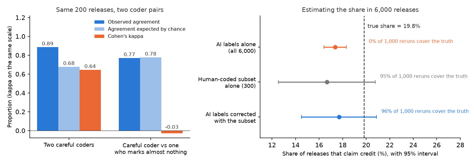
Read the left panel first. The careful pair agrees on 0.89 of the releases, and chance alone would have produced 0.68, so their kappa of 0.64 says they used a good part of the room above chance. Notice how modest 0.64 looks for two coders who are each right 95 percent of the time. That is the rare category at work: when most units are “no”, chance agreement is already high, and the same coders would earn a higher kappa on a category near half the corpus. So report the category’s share beside its kappa, and never compare kappas across categories as if prevalence did not matter (Feinstein and Cicchetti 1990). The second pair agrees on 0.77 of the releases, which sounds only a little worse. But chance alone predicts 0.78 for two coders with those habits, and the kappa of -0.03 says their agreement is entirely accidental. A value just below zero is chance noise around zero, not a meaningful disagreement: one of the coders marks the rare category only rarely, and at random. If you had reported percent agreement alone, you would have signed off on a coder who almost never marks the category you care about.
Now the right panel. The true share in this corpus is 19.8 percent. The AI labeler, run on all 6,000 releases, reports 17.4 percent with an interval from 16.4 to 18.3. That interval treats every label as correct. It is narrow because 6,000 is a large number, and it is wrong because the labeler misses a quarter of the real claims. Across the 1,000 reruns it covered the truth 0 percent of the time. More documents only made it more confidently wrong. The human-coded subset alone is honest but imprecise: 16.7 percent, from 12.5 to 20.8, covering the truth in 95 percent of reruns, which is what a 95 percent interval promises. The corrected estimate, 17.7 percent from 14.5 to 20.9, covered the truth in 96 percent of reruns with an interval narrower than the subset’s alone. Over 1,000 reruns, 96 percent is within noise of the promised 95. Both honest intervals also use the fact that the corpus is fixed: once you have coded 300 of its 6,000 releases, those 300 are no longer uncertain, which trims each interval slightly. In this one run both honest estimates happen to land below the truth, and both intervals still reach it. That is what an interval is for. In the companion notebook, raise the labeler’s catch rate from 0.75 to 0.95 and rerun. The corrected interval narrows further, because a better labeler leaves less error for the subset to repair. Watch the AI-alone share too: it now lands above the truth, because its false alarms among the 80 percent of ordinary releases outnumber the few claims it misses.
44.5 Where a text answer sits on the compass
A text project still answers to the inquiry compass, and the corpus frame decides its reach. If your question is how often these 6,000 releases claim credit, the estimand is a share of documents you hold, but you do not hold its answer. Humans applied the codebook to only 300 of them, so the 6,000 releases are the population your answer has to reach, and the crossing license is the random draw of the gold subset. That is why the corrected share carries an interval, and why the warrant is the codebook plus the gold-subset check. If your question is how often legislators in the state claimed credit in 2025, your population is every release they issued, and the answer needs a second crossing, from the retrieved archive to everything that was sent. That license is the one sampling gives you on the descriptive pathway. A retrieved archive is not a random sample of what was issued, so that license has to be argued: evidence that the releases you could retrieve stand in for the ones that went missing, or a bound on how far the missing ones could move your share.
Training a classifier to label future releases is a different inquiry. That is prediction, and it earns its reach only with the prediction-time honesty and the held-out check you met in the prediction chapter: documents the model never saw during training, ideally from a later period.
Two things words cannot license on their own. A count of credit-claiming releases describes what offices wrote, not what legislators privately believe or what they actually delivered. Documents are strategic: a press office writes for voters and reporters. And a rise in credit claiming after a new funding program is a description of timing, not a cause. If your question is causal, the text becomes your outcome measure inside a causal design, and the design, not the counting, has to carry the identification argument. “Causal, currently unidentified” stays a legitimate place to stop.
The same route runs through the book’s other domains. An economist codes the tone of central-bank statements, where the unit might be each policy paragraph and the frame is the bank’s own archive. A business analyst codes the risk language in companies’ annual reports filed with a securities regulator, where the frame is clean but firms copy last year’s wording, so repeated text is not new information. A biologist doing meta-research codes whether methods sections report how sample sizes were chosen, where the corpus frame is the set of journals searched and the gold subset protects against a keyword like “power” that means something else in a physiology paper. For a book-length treatment of these designs, Grimmer, Roberts, and Stewart set out the full framework (Grimmer et al. 2022).
44.6 An AI failure case
You paste ten press releases into a chatbot with your codebook and ask it to label each one and quote the sentence that justifies the label. It returns a clean table. Release 7 is marked “credit claiming” with the quote “I am proud to have brought $3 million home for our schools.” The table looks like evidence. You search release 7 for that sentence and it is not there. The release talks about a school-funding vote and never mentions an amount. The model produced a plausible quote to support the label it had already chosen. This is confident fabrication, the same failure that produces invented citations (Ji et al. 2023), now inside your measurement. A second failure waits one step later: you reword the prompt slightly, rerun the same ten releases, and three labels flip. That is prompt sensitivity: the labels depend on how the request was worded, so the definition of your category moved when the wording did, and nothing in the table tells you so.
A quote is a claim about a document. You catch the first failure by searching every quoted sentence in the source text, character for character, and treating any quote you cannot find as a failed label. You catch the second by freezing the prompt, recording the model version and date, and checking the labels against your gold subset each time anything changes. Then log both checks, and report the labeler’s error table beside the count it produced.
44.7 It is your turn
A further route beyond the five pathways. This lesson extends Studio 5: Develop the pathway. Read it once you have declared your primary pathway and your question calls for this design. Studio 5’s milestone asks for the same decisions, answered for this route.
You have a declared design and a pathway. This route is where a question answered from documents gets its corpus frame, its codebook, and its validation in writing, before any count is reported.
The hands-on half of this section lives in the chapter’s companion notebook: open it in Colab with the badge at the top, and work the steps there.
Commit your own answer first, then delegate. Each prompt is a checkable job, not a request for a verdict. Work them as a loop. The first answer is a draft: find the claim you cannot check, say so in your next message, and run it again. Some tools will label a whole corpus unattended and hand you a finished table. The finished look is exactly what makes the questions in this chapter worth asking before you accept it.
Three calls stay yours. You decide which documents count as your corpus and what the archive lost before you arrived. You decide what each label means, in a codebook you wrote, including the hard cases. And you decide whether a machine’s labels are good enough to count, on the evidence of your own human-coded subset. A tool can read, sort, and flag at a speed no person matches. You own the definition, the check, and the sentence that reports the count.
Write your corpus and its frame. In three lines, name the full body of documents your question is about, the collection you can actually retrieve, and who wrote those documents and why. Then list what may be missing and which way each gap could tilt your count.
When you are ready to delegate this step:
Act as an archivist. My question is about [the full set of documents]. The
collection I can retrieve is [your source, dates, how it was gathered]. List,
in a table, the kinds of documents likely missing from this collection, why
each went missing, and whether its absence would push my count up or down. Do
not tell me the collection is fine; I want the gaps.
After running, verify: check each named gap against what you know about how the archive was built, and confirm that the gap you wrote down first is on the list. Counters illusion of completeness (a tidy table that omits the one gap that matters most).
Fix your unit and write the codebook entry for your main category. Give the definition, at least two decision rules for hard cases, two examples, and two non-examples, all taken from your own documents.
When you are ready to delegate this step:
Here is my codebook entry: [paste it]. Act as a hostile second coder. Find
the five kinds of passages where two careful people applying this entry would
most likely disagree, and quote a made-up example of each, clearly labeled as
invented. Do not rewrite my definition; list the ambiguities so I fix them.
After running, verify: take each ambiguity to your own corpus and find a real passage that shows it; if every objection is mild, push back with “assume my definition is broken; name the worst case.” Counters sycophantic agreement (praise that reviews your ego, not your evidence).
Double-code a random subset and compute agreement yourself. Draw at least 50 units at random, and more if your main category is rare, because a kappa built on a handful of positive cases swings widely. Have a second person code them from the codebook alone, and report percent agreement, chance agreement, and Cohen’s kappa for your main category. Revise the codebook where you disagreed, and say so. If no second person is available, recode the same units yourself a week later without looking at your first labels, and report it as the weaker check it is.
When you are ready to delegate this step:
Act as a Python tutor. Here are two columns of labels from two coders on the
same units: [paste]. Explain, step by step, how to compute percent agreement,
the agreement expected by chance, and Cohen's kappa, and write the code. Show
the intermediate numbers so I can check each one by hand.
After running, verify: compute the three numbers by hand from your own two columns and confirm the code matches. A chance term that does not come from each coder’s own label rates, such as a flat 50 percent, is not Cohen’s kappa. Counters plausible-but-wrong method (a reliability number that looks standard and measures the wrong thing).
Validate any machine labeler against a human-coded gold subset before you count with it. Code a fresh random subset yourself, run the labeler on the same units with a frozen prompt, and report its misses and false alarms for each category. If you use its labels for a share, correct the share with the subset and report the interval.
When you are ready to delegate this step:
Apply this codebook exactly: [paste it]. Label each of the following
documents, and for every label give the one sentence from the document that
justifies it, copied word for word. If no sentence justifies a label, write
"no quote" instead of paraphrasing. [paste documents with their IDs]
After running, verify: search each quoted sentence in its source document, character for character, and count any quote you cannot find as a failed label. Counters confident fabrication (a quote invented to fit a label arrives as confidently as a real one).
Write the Research Contract lines for this route. State the question, the estimand (a share, a trend, or a difference, and in which documents), the data strategy (corpus frame, unit, sampling of the gold subset), the answer strategy (codebook, labeler, correction), the warrant that licenses its reach, and the limits: what the words cannot tell you about beliefs, deeds, or causes. If your question is not a text question, write one line saying which part of your project, if any, rests on documents, and whether its labels have been checked.
When you are ready to delegate this step:
Here is the claim I plan to report from my text analysis: "[paste your
sentence]." Act as a hostile reviewer. Name every word in it that claims more
than a count of documents can support, such as beliefs, intentions, effects,
or a population my corpus frame does not reach. Do not rewrite it for me.
After running, verify: check each flagged word against your estimand and frame, keep only the objections your design actually forces, and fix those yourself. Counters silent scope change (a count of what was written quietly upgraded to a claim about what people think or did).
Log the step in your AI Research Ledger, and verify at least one output with a named method from the Verification Guide. This route deserves two. Alternative code is the natural first check: recompute the labeler’s error table and the corrected share from your hand-coded subset by a second route, such as a spreadsheet, and land on the same numbers. Peer reasoning is the second: a second coder who reads only your codebook and disagrees with you on a case is evidence about the codebook, not about the coder. An AI reviewer may run the checks with you; the decision to accept or reject stays yours.