46 Evidence Synthesis: Scoping Reviews and Small Meta-Analyses
This chapter is part of a book in active development and has not yet been through the author’s review. Content may change as the review advances.

The research decision. Decide which studies count before you see a single result, how you will find every one of them, and whether combining them answers your question or only averages their biases. A tool can search, sort, and pool in seconds, but only you can defend why each study is in the pile and what the pooled number is allowed to mean.
46.1 Why this decision matters
The decision on the table: whether your pile of studies is a fair sample of the evidence, and whether one number can honestly speak for it.
“Tell me how a study got into your review before you tell me what the studies found. If you picked them after reading their results, your average is an opinion with a confidence interval attached.” — a review-journal methods editor, reading a manuscript that pooled twenty canvassing experiments into one estimate of persuasion
Once your question has been studied more than a few times, the most useful thing you can contribute may be a careful account of what those studies, taken together, actually say. That work has a trap built into it. A review can look exhaustive and still be a biased sample, because the studies that reach print are often the ones that found something. Pool a biased sample and you get a biased answer with a narrow interval, which is worse than no answer, because it looks settled. This chapter gives you the decisions that make a synthesis worth trusting, and the habit of saying exactly how far its number reaches.
46.2 The concept
Evidence synthesis sits in the complex-designs chapter of the design library in RDSS, which declares a meta-analysis as a design in its own right: the inquiry is the average of the true effects across studies and how much those true effects vary, and the answer strategy is a weighted average of the study estimates (Blair et al. 2023). That framing matters because it makes a review a research design with its own data strategy, not a reading list.
Evidence synthesis is the family of methods that answers a question by collecting, appraising, and combining the studies that already exist on it. Example: gathering every randomized experiment on door-to-door canvassing to ask how much a single conversation moves support for a candidate. It comes in two main shapes. A scoping review is a synthesis that maps what has been studied, how, where, and with which gaps, without pooling results into one number (Arksey and O’Malley 2005). Example: charting which countries, election types, and outcome measures the canvassing literature covers. A systematic review is a synthesis that answers a focused question with a prespecified search, explicit eligibility rules, an appraisal of each study, and often a pooled estimate (Higgins et al. 2024). Example: estimating the average effect of canvassing on turnout among randomized experiments published or posted before a fixed date.
Everything starts from a protocol, a written plan that fixes the question, the eligibility rules, the search, and the analysis before you screen anything. Example: a one-page document saying “randomized field experiments, any country, outcome is candidate support or turnout, searched in three named databases on a named date.” Researchers often frame the question with PICO (population, intervention, comparison, outcome) for effect questions, or PCC (population, concept, context) for scoping questions. Example: registered voters in general elections (population), a face-to-face canvassing visit (intervention), no visit (comparison), stated support for the candidate (outcome). Posting the protocol on a public registry such as the Open Science Framework before you start gives it a date stamp. The point is the same one that governs any design: decide what counts before the results can tempt you.
The data strategy of a review has four recorded steps. A search log is the exact record of where you searched, with which strings, on which dates, and how many records came back. Example: “Database X, 12 March, string canvass* AND (persua* OR vote choice) AND experiment*, 412 records.” Anyone should be able to rerun it. Screening is the two-stage filter that applies eligibility rules you wrote down before searching. Example: at the first stage you read titles and abstracts and send anything unclear forward; at the second you read full texts and give every study you exclude one reason from a list fixed in advance, such as “not randomized” or “no usable estimate.” The standard is two people screening every record without seeing each other’s calls. When that is out of reach, a second person screens at least a random share at each stage, and the agreement and how you settled each disagreement go in the log (Higgins et al. 2024). An AI tool can propose first-pass calls, but it is an assistant, not your independent second screener, and it never excludes a record nobody has read. Independence means two judgments made without seeing each other, and a person who reads the tool’s call before deciding tends to agree with it. The same split runs through the whole route. AI tools are fast at drafting search strings, removing duplicate records, proposing first-pass screening calls, and filling a draft extraction row. They are also known to invent studies that do not exist, to name databases as they were years ago, and to copy the wrong statistic from a crowded table (Ji et al. 2023). Every one of those outputs is a lead until you have opened the source yourself.
The PRISMA flow diagram is the standard chart of how many records you found, removed, screened, and kept, with the reason for every study excluded at full text (Page et al. 2021). It reports what you did. Its authors say plainly that PRISMA is a reporting guideline, not a tool for judging a review’s quality, so a tidy diagram certifies nothing about the studies inside it. Scoping reviews have their own reporting extension (Tricco et al. 2018). An extraction form is the fixed table you fill for every study: design, sample, setting, estimate, its uncertainty, and anything that threatens it. Example: one row per canvassing experiment, with the effect in percentage points and its standard error (how far the estimate would typically move if the study were run again on a new sample) copied from the study’s results table.
The form holds one row per study, and that rule needs defending. Dependent results are several estimates that come from the same study’s participants, so they rise and fall together. Example: one canvassing experiment that reports effects on candidate support and on turnout, at two survey waves, for two scripts compared against one shared control group. Entering those as separate studies counts the same households several times and makes the pooled interval narrower than the evidence. Write a rule in your protocol, before you extract, for choosing one estimate per study (for instance, the outcome the authors named as primary, at the longest follow-up), or combine the estimates within the study, or use a method built for dependent results (Higgins et al. 2024; Borenstein et al. 2021).
Two appraisal steps come next. Risk of bias is your study-by-study judgment of whether the design and conduct could have tilted the result. Example: an experiment that lost a third of its households before the follow-up survey gets flagged. Rating the certainty of the evidence is the final judgment of how much trust the whole body deserves, weighing risk of bias, inconsistency, indirectness (studies that answer a slightly different question from yours), imprecision, and missing studies (Higgins et al. 2024). Example: six well-run experiments that agree earn more trust than twenty small ones that scatter.
Then, if pooling is defensible, the answer strategy. An effect size is each study’s result expressed on one shared scale, so studies can be compared. Example: every canvassing effect converted to percentage points of support. A meta-analysis is the statistical combination of those effect sizes into one weighted average with an interval (Borenstein et al. 2021). The weights come from inverse-variance weighting, which means each study counts in proportion to its precision. Example: a study of 20,000 households with a standard error of 0.45 points counts about ten times as much as one with a standard error of 1.4 points. Two models set what the average means. A fixed-effect model assumes every study estimates one identical true effect and differs only by chance. Example: six replications of the same script, in the same kind of district, in the same kind of election. A random-effects model assumes each setting has its own true effect and estimates their average and their spread. Example: canvassing in different countries and years, where a conversation may simply matter more in some places. Heterogeneity is the disagreement among studies beyond what chance alone would produce. Example: canvassing moving votes in primaries and ballot-measure campaigns but not in general elections (Kalla and Broockman 2018). A forest plot is a chart that shows each study’s estimate and interval on one row, with the pooled estimate as a diamond at the bottom. Example: the left panel of the figure later in this chapter.
One habit to drop now. Vote counting means tallying how many studies were statistically significant (an estimate far enough from zero that chance alone rarely produces it) and calling the majority the answer. It misleads because a small study can miss a real effect, so “most studies found nothing” can describe a literature of small studies that all point the same way (Borenstein et al. 2021).
Now the compass. The kind of a synthesis question comes from its words, as for any other question. “How much does a canvassing visit change support for the candidate?” is causal whether your pile holds randomized experiments or observational comparisons. The designs decide what the answer can establish. A pooled average of randomized experiments carries their assignment license to a causal claim. A pooled average of observational comparisons does not: the question stays causal, that pile leaves it currently unidentified, and the claim you can make is an association unless each study defends its own identification. Pooling never creates a crossing license. The synthesis inherits each study’s warrant, and averaging twenty confounded comparisons gives you one confounded comparison with a smaller interval. Reach needs care too. A pooled effect question reaches for a population: the settings where the intervention could be used. The studies you pooled were not sampled at random from those settings, so no sampling license carries the average there. The random-effects average describes settings like those that were studied and reported, and saying more requires an argument about which settings are missing. A scoping review asks a descriptive question whose population is every eligible study, including the ones your search did not find: what has been studied, how, and where. Its warrant is the completeness of your search, which the search log documents and a missed database weakens, and it makes no claim about what the true effect is. This route builds on the search habits of Finding and Verifying Prior Evidence, and it is a multi-part design in the sense of Hybrid and Complex Designs: each stage of the review carries its own error into the final number.
46.3 A worked example
Bring this into political science. A campaign asks you whether its volunteers should keep knocking on doors to persuade voters in a general election. You find six randomized canvassing experiments that meet your protocol (these six are constructed for the example). Five of them report effects too imprecise to call significant, and one reports a clear positive effect. A quick reader says “five of six found nothing, so canvassing does not persuade.” That is vote counting, and it is not the evidence talking.
Pool them instead. Each study’s estimate goes in with a weight set by its precision, so the large study E, with a standard error of 0.45 points, carries the most weight. The fixed-effect average comes out at about 0.6 of a point, with an interval running from just below zero to about 1.25 points. The random-effects average is almost the same, because the six studies disagree little beyond chance: the share of their spread that exceeds chance is only 7 percent. Treat that 7 percent loosely. With six studies, the spread between settings is estimated very poorly, and the usual random-effects interval, built on the normal curve, tends to come out too narrow when studies are this few (Higgins et al. 2024). The Hartung-Knapp-Sidik-Jonkman interval is the random-effects interval built for that case: it scales the uncertainty to how much the studies actually scatter and uses a wider multiplier from the t distribution, which allows for estimating the spread from few studies. Example: with six studies the multiplier is about 2.57 instead of 1.96. It is the interval the code below reports, and the reading it supports is modest: the pooled evidence is consistent with a small positive average effect, cannot distinguish it from zero, and makes an average effect above about 1.6 points unlikely for settings like these.
Political scientists have run this synthesis for real. Kalla and Broockman pooled 40 field experiments and added nine of their own, and concluded that the best estimate of campaign contact’s persuasive effect in United States general elections is zero, a finding that sets a sober prior for any campaign reading your review (Kalla and Broockman 2018).
The block below pools the six constructed studies both ways, counts the votes, and then repeats the pool after one extraction slip. Watch what happens to the interval when one number lands in the wrong column.
import numpy as np, pandas as pd
from scipy import stats

# Six canvassing experiments, CONSTRUCTED for this example. Each row is one
# study's effect on support for the candidate (percentage points) and its
# standard error, copied from the study's own results table. One row per study:
# where a study reported several estimates, the protocol's rule picked one.
studies = pd.DataFrame({
    "study":    ["A", "B", "C", "D", "E", "F"],
    "estimate": [2.9, 0.6, -0.4, 2.4, 0.3, 1.1],
    "se":       [1.4, 0.8, 1.1, 1.7, 0.45, 0.9],
})

def pool(y, s):
    k = len(y)
    w = 1 / s**2                                   # precise studies weigh more
    fixed = np.sum(w * y) / np.sum(w)
    fixed_ci = fixed + np.array([-1.96, 1.96]) / np.sqrt(np.sum(w))
    q = np.sum(w * (y - fixed) ** 2)               # disagreement beyond chance?
    tau2 = max(0.0, (q - (k - 1)) / (np.sum(w) - np.sum(w**2) / np.sum(w)))
    wr = 1 / (s**2 + tau2)                         # weights that allow for the spread
    rand = np.sum(wr * y) / np.sum(wr)
    se_z = 1 / np.sqrt(np.sum(wr))
    z_ci = rand + np.array([-1.96, 1.96]) * se_z   # normal approximation: too narrow
    # Hartung-Knapp-Sidik-Jonkman: rescale by the scatter the studies show (never
    # below the usual standard error) and use a t multiplier on k - 1 df.
    scatter = np.sum(wr * (y - rand) ** 2) / (k - 1)
    se_h = np.sqrt(max(scatter, 1.0)) * se_z
    hk_ci = rand + np.array([-1, 1]) * stats.t.ppf(0.975, k - 1) * se_h
    # Prediction interval: where the true effect in ONE new setting may fall.
    pred = rand + np.array([-1, 1]) * stats.t.ppf(0.975, k - 2) * np.sqrt(tau2 + se_z**2)
    i2 = max(0.0, (q - (k - 1)) / q) * 100
    return dict(fixed=fixed, fixed_ci=fixed_ci, rand=rand, hk_ci=hk_ci,
                z_ci=z_ci, pred=pred, i2=i2)

def show(ci):
    return f"[{ci[0]:+.2f}, {ci[1]:+.2f}]"

y, s = studies.estimate.to_numpy(), studies.se.to_numpy()
sig = (np.abs(y / s) > 1.96).sum()
r = pool(y, s)
print(f"vote count (significant studies)  : {sig} of {len(y)}")
print(f"fixed-effect pooled estimate      : {r['fixed']:+.2f}  {show(r['fixed_ci'])}")
print(f"random-effects pooled estimate    : {r['rand']:+.2f}  {show(r['hk_ci'])}")
print(f"  same, normal-approximation CI   :        {show(r['z_ci'])}")
print(f"prediction interval, new setting  :        {show(r['pred'])}")
print(f"share of spread beyond chance (I2): {r['i2']:.0f}%")

# One extraction slip: study E's outcome STANDARD DEVIATION (48 points, from
# its descriptive table) typed into the standard-error column.
s_bad = s.copy(); s_bad[4] = 48
b = pool(y, s_bad)
print(f"\nsame pool, E's SD typed as its SE : {b['rand']:+.2f}  {show(b['hk_ci'])}")
print(f"  with the normal-approximation CI:        {show(b['z_ci'])}")
print("the largest study vanished from the average and nothing crashed")
The printout gives a fixed-effect estimate of +0.61 points with an interval of -0.03 to +1.25. The random-effects estimate is +0.65, and its Hartung-Knapp-Sidik-Jonkman interval runs from -0.27 to +1.57, wider than the -0.04 to +1.35 the normal approximation would claim. The campaign, though, is deciding about its own next election, a setting none of the six studied. A prediction interval is the range where the true effect in one new setting is likely to fall, allowing for both the uncertainty in the average and the spread between settings. Example: the printout’s -0.56 to +1.86, which says the next election could see a small backfire, no persuasion, or close to two points. With six studies that range is itself rough, but it is the range the campaign’s decision needs (Higgins et al. 2024).
The last lines are the warning. With study E’s standard deviation typed where its standard error belonged, the largest study nearly disappears from the average and the random-effects estimate jumps from +0.65 to +0.95, while the code runs without complaint. The Hartung-Knapp-Sidik-Jonkman interval, -0.26 to +2.17, still spans zero. Report the same pool with the normal approximation, as many default tools do, and you get +0.03 to +1.88, which excludes it. Two routine-looking errors, one wrong cell and one interval too narrow for six studies, together turn “cannot tell from zero” into “persuades.”
46.4 A seeded simulation
A review can be flawless in every step you control and still inherit a bias you cannot see: the studies that never reached print. The code below builds a world where 30 canvassing experiments are run and the true average effect is 1.0 point. Every study with a significant positive result gets published. Each of the others gets out only by luck, one time in four. Then it pools the published studies the way a careful reviewer would, and pools all 30 the way nobody can. The seed makes the run reproduce this exact figure.
import numpy as np
import matplotlib.pyplot as plt
from scipy import stats

SEED = 464
rng = np.random.default_rng(SEED)

k, mu, tau = 30, 1.0, 0.5            # 30 studies RUN; true average +1.0 point
se = rng.uniform(0.3, 2.5, k)        # small studies carry large standard errors
theta = rng.normal(mu, tau, k)       # each study's own true effect
est = rng.normal(theta, se)          # what each study reports
significant = est / se > 1.96
published = significant | (rng.random(k) < 0.25)   # nulls rarely get out

def pool(y, s):                      # random-effects average, HKSJ interval
    k = len(y)
    w = 1 / s**2
    fe = np.sum(w * y) / np.sum(w)
    q = np.sum(w * (y - fe) ** 2)
    t2 = max(0.0, (q - (k - 1)) / (np.sum(w) - np.sum(w**2) / np.sum(w)))
    wr = 1 / (s**2 + t2)
    m = np.sum(wr * y) / np.sum(wr)
    scatter = np.sum(wr * (y - m) ** 2) / (k - 1)
    half = stats.t.ppf(0.975, k - 1) * np.sqrt(max(scatter, 1.0) / np.sum(wr))
    return m, m - half, m + half

all_m, all_lo, all_hi = pool(est, se)
pub_m, lo, hi = pool(est[published], se[published])
print(f"published: {published.sum()} of {k}, significant: {significant.sum()}")
print(f"pooled, all run   : {all_m:.2f} [{all_lo:.2f}, {all_hi:.2f}]")
print(f"pooled, published : {pub_m:.2f} [{lo:.2f}, {hi:.2f}]")

fig, (a1, a2) = plt.subplots(1, 2, figsize=(9.6, 4.2))
idx = np.where(published)[0]
idx = idx[np.argsort(se[idx])]                     # most precise on top
ys = np.arange(len(idx), 0, -1) + 1.0
a1.errorbar(est[idx], ys, xerr=1.96 * se[idx], fmt="s", color="#2a78d6", ms=4)
a1.fill([lo, pub_m, hi, pub_m], [0.5, 0.85, 0.5, 0.15], color="#eb6834")
a1.axvline(0, color="#9a9a9a", lw=0.8)                 # zero effect
a1.axvline(mu, color="#333333", ls="--")               # the truth
a1.set_xlabel("Effect on support (percentage points)")
a1.set_title("What the published record shows", loc="left")
a2.scatter(est[published], se[published], color="#2a78d6", label="published")
a2.scatter(est[~published], se[~published], facecolors="none",
           edgecolors="#9a9a9a", label="never published")
grid = np.linspace(0, se.max() * 1.05, 50)
a2.plot(1.96 * grid, grid, color="#9a9a9a", ls=":", label="significance line")
a2.axvline(pub_m, color="#eb6834", label="pooled, published")
a2.axvline(all_m, color="#2a78d6", label="pooled, all run")
a2.axvline(mu, color="#333333", ls="--"); a2.invert_yaxis()
a2.set_xlabel("Effect on support (percentage points)")
a2.set_ylabel("Standard error"); a2.legend()
a2.set_title("Every study that was run", loc="left")
plt.show()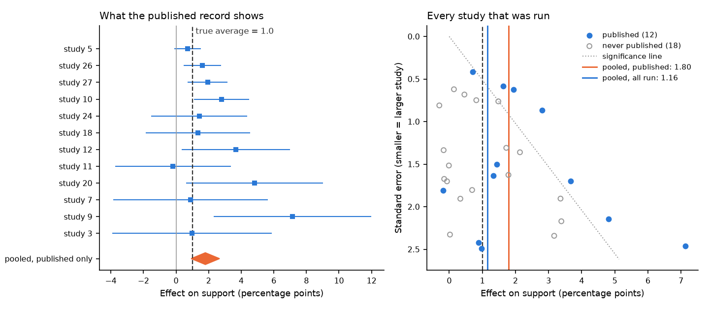
Read the left panel first, because it is all a reviewer ever sees. Twelve published studies, most intervals overlapping, and a pooled diamond at 1.80 points with an interval from 0.93 to 2.67. Half the rows are significant and half are not, so a vote counter would call the literature split. The pooled estimate says something firmer and wrong: an effect near 1.8 points, with the true average of 1.0 only just inside the lower tip of its interval.
Now the right panel, which no real reviewer can draw. It is a funnel plot, a scatter of each study’s estimate against its standard error, with the most precise studies at the top. Without a publication filter the dots would spread evenly around the true average, narrowing toward the top like an upturned funnel. Here the 18 hollow circles that never reached print all sit left of the dotted significance line, and most of them report less than the true 1.0 point. Remove them and the published dots lean to the right, toward large positive effects. Pool all 30 and you get 1.16 points, with an interval from 0.72 to 1.60 that contains the truth. Pool the published 12 and the estimate is about 55 percent larger. The size of the pile did not cause this. The filter did: publication bias, the tendency of results to reach print because of what they found.
A lopsided funnel is a warning light, not a diagnosis. Asymmetry can also come from small studies that were run in different settings, from poor design in small studies, or from chance, and the standard advice is to test for it only when at least ten studies are pooled (Sterne et al. 2011; Egger et al. 1997). When you see it, you say so, you search harder for unpublished work (registries, preprints, conference programs, emails to authors), and you report how the pooled estimate changes when you pool only the larger, more precise studies. In the companion notebook, change the 0.25 to 1.0 so every null is published, rerun, and watch the two vertical lines converge.
46.5 When one number is the wrong answer
Pooling is a choice, and often the right choice is not to make it. Four situations call for a scoping review or a structured narrative synthesis instead.
The studies answer different questions. An economist reviewing cash-transfer programs finds studies of unconditional grants, school-conditional grants, and transfers paired with training. One average across them answers none of the three questions a policymaker would ask.
The studies carry different warrants. A business analyst might hold a company’s randomized product tests beside its before-and-after comparisons of the same features. The randomized tests have a causal license; the before-and-after comparisons do not, and pooling them hands the weaker design the stronger design’s credibility.
The outcomes cannot share a scale. An ecologist synthesizing predator-removal experiments may find prey counts, biomass, and survival rates. Standardized effect sizes can put some of these on one scale, but only when you can defend that they measure the same thing (Koricheva et al. 2013; Gurevitch et al. 2018).
The heterogeneity is the finding. When canvassing works in primaries and not in general elections, the average of the two is a number that describes no election. Report the split, and treat the reason for it as the next question.
In each case the honest product is a map: a table of what was studied, in which settings, with which designs and outcomes, and where the gaps sit. That map is a real contribution, and it is often the one a first synthesis should aim for.
46.6 An AI failure case
You paste the six study PDFs into an AI tool and ask it to fill your extraction form and pool the results. It returns a clean table and a confident paragraph: “The pooled effect is +0.95 points (95% interval +0.03 to +1.88), indicating that canvassing reliably increases candidate support.” Every row looks plausible. But in one row the tool copied the outcome’s standard deviation from a descriptive table into the standard-error column, it built the interval on the normal approximation that six studies cannot support, and its paragraph cites a seventh, “confirming” study by a real-sounding author team that appears in none of your PDFs. This is two named failures at once: confident fabrication, a citation and a number that no source contains, and silent scope change, “cannot tell from zero” quietly upgraded to “reliably increases.” A tidy table is not an extraction. You catch it by tracing every cell back to a page: open each PDF, find the table the number came from, and confirm it is the standard error, not the standard deviation. Delete any citation you cannot open. Then rerun the pool on your verified table with the Hartung-Knapp-Sidik-Jonkman interval, write the sentence that interval licenses, and log why the tool’s version was rejected.
46.7 It is your turn
A further route beyond the five pathways. This lesson extends Studio 5: Develop the pathway. Read it once you have declared your primary pathway and your question calls for this design. Studio 5’s milestone asks for the same decisions, answered for this route.
Your question has a literature, and you have chosen to make that literature your data. This step writes the review’s own Research Contract, so every study in your pile has a documented reason to be there.
The hands-on half of this section lives in the chapter’s companion notebook: open it in Colab with the badge at the top, and work the steps there.
Commit your own answer first, then delegate. Each prompt is a checkable job, not a request for a verdict. Work them as a loop. The first answer is a draft: find the claim you cannot check, say so in your next message, and run it again. Some tools will run that whole loop unattended and hand you a finished review. The finished look is exactly what makes the questions in this chapter worth asking before you accept it.
Three calls stay yours. You decide which studies are eligible, in writing, before you read any result, because a rule set after the results is a filter on the answer. You decide whether pooling is defensible at all, because only you can judge whether the studies answer one question with comparable designs and outcomes. And you decide what the synthesis can claim, since it inherits every study’s warrant and no more. A tool can search, screen a first pass, and compute a weighted average in seconds. You own the eligibility rules, the decision to pool, and the sentence that reports it.
Write your review question and its eligibility rules before you search. Use PICO for an effect question or PCC for a scoping question, and add the designs you accept, the date range, the languages, the reasons you will use to exclude a full text, and your rule for choosing one estimate when a study reports several. Then write your Research Contract lines for this route: the question; the estimand (the average true effect and its spread, or for a scoping review the map you will produce); the data strategy (search, screening, extraction); the answer strategy (pooling or a structured narrative); the warrant (the studies’ own crossing licenses, never the pooling); and the limits (which settings and which unpublished work you may be missing).
When you are ready to delegate this step:
Act as a systematic-review methodologist. Here is my review question and my
eligibility rules: [paste them]. List, as a table, every term in my rules that two
careful screeners could read differently, and for each one give an example study
that one would include and the other would exclude. Do not rewrite my rules for me.
After running, verify: read each flagged ambiguity against your own question and tighten only the rules where the example would really split two screeners. If the tool finds no ambiguity at all, ask again with “assume two screeners disagree on 10 percent of records; which rule causes it?” Counters illusion of completeness, a tidy table that implies your rules have no gaps.
Build a search log you could hand to a stranger. Name each database or source, the exact search string, the date, and the number of records it returned, and add at least one route to unpublished work.
When you are ready to delegate this step:
Act as a research librarian in political science. My review question is
[paste it]. Suggest the databases and registries where studies on it are indexed,
and draft one search string for each using its own syntax. Only name databases
you are confident exist; mark anything uncertain.
After running, verify: run every string yourself, record the hit count and date in your log, and drop any database you cannot open. Counters stale knowledge (a database renamed, merged, or retired since the tool learned about it).
Screen in two stages with the rules you fixed in step 1. At titles and abstracts, send anything unclear forward. At full texts, give every excluded study one reason from your list and log it. Then make a documented second check: ideally a second person screens every record, and at minimum a random 20 percent at each stage, blind to your calls, and you log the agreement and how each disagreement was settled. If no second person is available, say in your report that one person screened. Before a tool proposes calls on anything, test it on a random sample you have already screened blind, and never let it exclude a record you have not read.
When you are ready to delegate this step:
Here are my eligibility rules [paste them] and 50 titles and abstracts [paste
them]. For each record, say include, exclude, or unsure, and quote the exact words
in the abstract that decided it. Do not decide a record from its title alone.
After running, verify: compare the tool’s calls with the ones you made blind, and read every disagreement in full. Record the agreement rate in your log, and count the eligible records the tool would have excluded: if there are any, use it only to order your reading, never to exclude. Counters correlated errors, a checker who reads the tool’s answer first and inherits its mistakes.
Extract every study onto one form and trace each number to a page. For each study, record the design, the setting, the estimate, its standard error or interval, and your risk-of-bias note, with the page and table where each number sits. Keep one row per study: when a study reports several estimates for your question, apply the rule from step 1 and list the others in a note, never as new rows.
When you are ready to delegate this step:
Act as a careful research assistant. From the attached study, fill this extraction
form: [paste the form]. For every number, give the page and table it came from and
say whether it is a standard error, a standard deviation, or a confidence interval.
If a field is not reported, write "not reported"; never estimate it.
After running, verify: open the page cited for every number and confirm it exists, says that, and is the quantity the column asks for. Counters confident fabrication, a number or a study that appears in no source you can open.
Decide whether to pool, and write the synthesis sentence. If you pool, report the pooled estimate with an interval built for few studies (the Hartung-Knapp-Sidik-Jonkman interval), a prediction interval if you have at least five studies, the heterogeneity, and your funnel-plot note; if you do not, write the map and one sentence on why one number would mislead. Either way, name the warrant the studies carry and the settings the answer reaches. If you found only a handful of eligible studies, or they disagree on design and outcome, the map is your product.
When you are ready to delegate this step:
Here is my synthesis sentence: "[paste it]" and the studies behind it: [paste the
extraction table]. Act as a hostile review-journal editor. List every word that
claims more than these designs, this interval, and these settings allow. Do not
rewrite the sentence for me.
After running, verify: check each flagged word against the studies’ own designs and your interval, and keep only the objections the evidence forces. If every objection is mild, push back with “assume the sentence is wrong; name the single worst flaw.” Counters sycophantic agreement (praise that reviews your ego, not your evidence).
Log the step in your AI Research Ledger, and verify at least one output with a named method from the Verification Guide. Primary-source reading is the natural check for this route: open the PDF behind every extracted number. Direct calculation is the strong second check: recompute the pooled estimate by hand from your verified table and land on the same number. An AI reviewer may run the checks with you; the decision to accept or reject stays yours.