20 Data Provenance and Data Quality
This chapter is part of a book in active development and has not yet been through the author’s review. Content may change as the review advances.

The research decision. For every number, dataset, and source your project leans on, decide whether it is solid enough to build on. You make that call twice: once on where the value came from and whose hands it passed through, its provenance, and once on whether it was produced well enough, under the right definition, for the specific use you have in mind, its quality.
20.1 Why this decision matters
The decision on the table: whether a number you did not produce yourself is solid enough to carry your project’s weight.
Picture an advisor, the researcher who will eventually sign off on your project, reading the first draft of your background section:
“You wrote that turnout in this county was 72 percent. Where did that come from? Not which website you copied it off. Who counted the ballots, and 72 percent of what? Of registered voters, of adults, of adults actually eligible to vote? Bring me the office that certified the count, or take the number out.”
A value with no traceable origin is a rumor with a decimal point. Precision is not the same as trust. This chapter trains you to stop treating a number or a citation as true because it arrived looking tidy, and to ask two questions of everything you borrow: where did it come from, and is it any good for what I need it for.
20.2 The concept
Data provenance is the documented origin of a value and every hand it passed through before it reached you (Lebo et al. 2013) (Wilkinson et al. 2016). Example: a turnout figure in a news story, traced back through a state summary table to the county election office that certified the count.
That chain has two kinds of links. A primary source is the original record where a value was first produced. Example: the county’s certified canvass, the official document reporting the final vote totals. A secondary source re-reports a value it did not produce. Example: a newspaper table, an encyclopedia entry, or a data aggregator that copies the county’s number. A value is only as trustworthy as the primary source at the end of its chain.
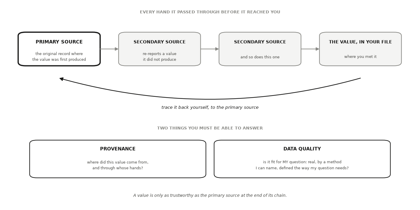
Data quality is whether a value is fit for your specific use: real, produced by a method you can name, and defined the way your question needs (Wang and Strong 1996). Example: a turnout rate computed over registered voters is high quality for a question about whether registered people showed up, and the wrong number for a question about how much of the adult population takes part. A mischaracterized value is a real number attached to the wrong definition or method. Example: a survey’s self-reported turnout presented as an official count, or a registered-voter rate cited as though it covered everyone eligible.
Whole datasets carry the same two questions, column by column. Who produced this variable, who cleaned it, what did they drop, and does the definition behind the column match the one in your question? A file that lands in your folder with no answers to those questions is not yet data. It is a rumor in a spreadsheet.
You settle all of it with one habit, the retrieval-verification loop: Ask a tool to surface a value and its source, Retrieve the primary source yourself, Verify that it exists and reports that value under that definition, and Document where you found it. A citation you have not opened is a lead, not a source, however confident the tool that handed it to you.
20.3 A worked example
Suppose you are studying whether a local election reform changed participation, and you need one number to anchor your background section: turnout in a particular county in a recent presidential election. You ask an AI assistant and get an answer in about a second. Seventy-two percent, with a source that looks entirely real.
You run the loop instead of copying the number. First, provenance. You search the exact title of the source. If it resolves nowhere, the value is orphaned and you drop it. If the page is real, you ask whether it produced that number or merely republished it. That question usually sends you one link further back, to the state’s official results summary, and behind that to the county clerk’s certified canvass, which is where the totals were actually settled.
Then, quality. You open the canvass and read what the percentage is of. Is the denominator registered voters, all adults, or adults eligible to vote, which excludes noncitizens and, in some states, people with certain felony convictions? Those three denominators produce three different turnout numbers for the same election, and the gaps between them are not small. You also ask whether the figure was counted or estimated. Ballots cast are counted. Eligible-population denominators are estimated from census data. Survey turnout is self-reported, and people reliably overstate whether they voted, so it is a third kind of number again.
You cross-check against an independent source that documents its own methods. Two worth knowing: the United States Elections Project, which publishes voting-eligible-population turnout estimates and explains exactly how it builds the denominator, and the Census Bureau’s Current Population Survey Voting and Registration Supplement, which reports self-reported turnout from a large national survey. When the certified canvass and an independent reference agree on both the count and the definition, the number has earned a place in your project. When they disagree, the disagreement is the finding. You report both, name the definition behind each, and say which one your question needs and why.
That a value’s usefulness depends on its documented origin and on fitness for the specific use, not on precision alone, is the standard framing of data quality (Wang and Strong 1996).
The block below is not a simulation. It is the same numerator divided by the three denominators a real turnout figure might be resting on, so you can see how much of the answer the label decides.
import pandas as pd
SEED = 464   # no random draw here: provenance is a chain, not a sample

# One county, one election, three denominators — each a real kind of published
# figure, each answering a different question. Replace these with the numbers
# you retrieve from the canvass and the census table you name.
ballots_cast = 214_318
denominators = {
    "registered voters (clerk's canvass)": 297_664,
    "voting-age population (census estimate)": 341_902,
    "voting-eligible population (estimate)": 312_540,
}
rows = [{"denominator": k, "count": v,
         "turnout %": round(ballots_cast / v * 100, 1)}
        for k, v in denominators.items()]
print(pd.DataFrame(rows).to_string(index=False))
print(f"\nspread across the three : "
      f"{max(r['turnout %'] for r in rows) - min(r['turnout %'] for r in rows):.1f} "
      f"percentage points")
print("one election, one numerator, three published turnout numbers.")
print("a figure with no stated denominator is not yet evidence")
20.4 Missing data: the rows you do not see
Suppose the county’s election office also mails a short follow-up survey to 4,000 registered voters, drawn at random from its list, asking whether they voted. About six in ten send it back. Your file has 4,000 rows, but the turnout column is blank in roughly 1,600 of them. Every summary you compute from that file quietly describes the people who answered, unless you decide otherwise and say how.
Missing data are values that should exist in your file but do not. Example: a respondent who skipped the income question, a field sensor that failed for a week, or a firm that never filed one quarter’s report. Ask of every blank what you ask of every value: who dropped it, and why. The answer decides what you can claim.
Researchers sort those reasons into three mechanisms, a classification that goes back to Rubin (Rubin 1976) and that later textbooks built into everyday practice (Little and Rubin 2019; Buuren 2018).
- Missing completely at random means the chance a value is missing has nothing to do with anything, measured or not. Example: a lab technician drops one tray of samples picked by accident. You lose precision, but the answer does not tilt.
- Missing at random means the chance a value is missing depends only on things you did observe. Example: younger voters return the survey less often, and the voter file tells you everyone’s age. You then assume that, within an age group, the people who answered vote like the people who did not.
- Missing not at random means the chance a value is missing depends on the missing value itself. Example: people who stayed home on election day are less likely to return a survey about voting. No column in your file measures that gap.
Complete-case analysis means computing your result only from the rows with no blanks. Example: averaging a column by skipping its empty cells, as most software does by default. When values are missing completely at random it gives an unbiased answer, only a less precise one. Under the other two mechanisms it can tilt the answer, though not always: if the blanks in an outcome depend only on the explanatory variables in a regression, the slopes fitted to the complete rows can still be right (Little and Rubin 2019). A plain average of the outcome, like county turnout, has no such protection.
Your first move is descriptive. A missingness table is the share of blank values broken down by groups you can observe. Example: 74 percent of older voters answered and 46 percent of younger voters did. The table cannot reveal whether the non-answerers differ in the value you care about. It does show the blanks are spread far more unevenly than chance would produce, so the first mechanism is not your situation.
Imputation means filling each blank with a value predicted from what you did observe. Example: give each non-answerer the turnout rate of answerers in the same age group. It removes the whole tilt only when the values are missing at random given the variables it uses and the model that fills them includes every variable your later analysis will use. Short of that, it can repair the part of the tilt that runs through variables you measured and leaves the rest in place. Multiple imputation fills each blank several times with plausible values and combines the results. Example: twenty filled-in copies of the survey file, analysed one by one and pooled. It carries the uncertainty of the guess into your interval (Buuren 2018). No method recovers information your file never held: if the values are missing not at random, the filled-in values inherit the tilt. And a single fill, like the one in the example, treated as real data makes your interval narrower than your knowledge, because the file now pretends the guesses were observed.
So you add a check that needs no assumption about the blanks. Bounds are the lowest and highest values your answer could take under the most extreme possibilities for the missing rows, which you can compute whenever the value has natural limits, like a yes-or-no vote. Example: turnout if every non-answerer stayed home, and turnout if every one of them voted (Manski 1989). Bounds are often wide, and that width is exactly what your missing rows cost you.
The block below builds a constructed county where you can see the true turnout, something you never get in practice. Answering depends on age, which the file records, and on voting itself, which it does not.
import numpy as np, pandas as pd
SEED = 464
rng = np.random.default_rng(SEED)

# 4,000 registered voters drawn at random from one county's list.
# Older people vote more often.
n = 4_000
older = rng.random(n) < 0.5
voted = rng.random(n) < np.where(older, 0.75, 0.50)
# Who answers the follow-up survey? Older people answer more, AND people
# who voted answer more than people who did not: the missing value itself.
answered = rng.random(n) < 0.35 + 0.20 * older + 0.25 * voted

df = pd.DataFrame({"group": np.where(older, "older", "younger"),
                   "voted": voted, "answered": answered})
print(df.groupby("group")["answered"].agg(people="size", share_answered="mean").round(2))

seen = df[df.answered]
missing = (~df.answered).sum()
complete_case = seen.voted.mean()
# Fill each blank with the turnout of answerers in the same age group.
rate = seen.groupby("group").voted.mean()
filled = df.voted.where(df.answered, df.group.map(rate)).mean()
low = seen.voted.sum() / n                 # every non-answerer stayed home
high = (seen.voted.sum() + missing) / n    # every non-answerer voted

print(f"\nshare of rows missing                 : {missing / n:.3f}")
se = np.sqrt(complete_case * (1 - complete_case) / len(seen))
print(f"complete-case turnout                 : {complete_case:.3f}"
      f"  (95% interval {complete_case - 1.96 * se:.3f} to {complete_case + 1.96 * se:.3f})")
print(f"filled in by age group                : {filled:.3f}")
print(f"bounds with no assumption at all      : [{low:.3f}, {high:.3f}]")
print(f"true turnout of all 4,000 (unseen)    : {df.voted.mean():.3f}")
print("\nfilling in by age repairs the age part of the gap, not the voting part;")
print("only the bounds hold whatever the non-answerers did")
Read the output against the true value of 62.4 percent. With 40.2 percent of the rows blank, the complete-case turnout is 73.9 percent, and its 95 percent interval, 72.2 to 75.7, misses the truth: that interval measures sampling noise among the people who answered, not who stayed silent. Filling in by age group moves it to 71.9 percent, about two points repaired and 9.5 points still wrong, because the rest of the tilt runs through voting itself. The bounds run from 44.2 to 84.4 percent, a width of 40 points that equals the share of missing rows. They contain the truth, and they would contain it whatever the non-answerers did.
Your estimand is turnout among all registered voters in the county, not among the people who returned the form. The random draw gives you the sampling license from 4,000 voters to the county, but nonresponse breaks it unless you defend an assumption about why rows went missing, and nothing in the file can confirm that assumption. The bounds cover only the blanks among the 4,000; carried to the county, each end also needs a sampling interval. So you report a filled-in estimate, from multiple imputation so its interval carries the guess, with its assumption written beside it, the bounds as a sensitivity check, and one outside benchmark. In a real county the certified canvass counts the ballots, and a survey figure far above it warns you about who answered and about people overstating that they voted. When the blanks are outcomes in an experiment, the same logic returns as attrition on the experimental-causal pathway.
An AI tool writes the missingness table, the imputation code, and the bounds in seconds. Two habits keep it honest. Ask it to print the number of rows before and after every step, because code tools often drop incomplete rows or fill blanks with a column average without telling you, a silent scope change from all 4,000 voters to the ones who answered. And treat any sentence like “the data are missing at random” as your claim to defend, since it is a statement about people you never heard from. When values go missing or come back false because the question is sensitive, you can sometimes redesign the question instead: the survey experiments route shows how a list experiment lets people answer without revealing their own answer.
20.5 An AI failure case
You ask for county turnout and the tool returns “72 percent,” with a citation to a real state elections page. Seven details look right, so it is tempting to paste it straight in. You open the page instead, and the table header reads percent of registered voters, not percent of everyone eligible. The number is real. The denominator is the wrong one for your question, and the tool swapped it silently. You catch it two ways. You had written your own expectation first, so a figure that sits well above what you knew about participation in that county already looked suspect. Then you read the actual column header rather than the tool’s summary of it, and the mismatch is plain. The value goes into your notes as a registered-voter rate, and your original question stays open.
20.6 It is your turn
You are working inside Studio 6: Govern data and measurement. Keep what you write here; the studio’s milestone chapter is where it joins the other lessons’ pieces into one artifact you can defend.
Your pathway is declared and your contract remains provisional; your measurements come next. Before either can be trusted, this step pins down where your data actually came from.
The hands-on half of this section lives in the chapter’s companion notebook: open it in Colab with the badge at the top, and work the steps there.
Each prompt is commit-first: write down the value or source you already believe, then let the tool disagree with something of yours. Treat every one as the start of a loop rather than a single request. The first answer gives you leads; your second message names the lead that did not survive retrieval and asks again. Tools that run the search loop on their own will hand you a longer, tidier list of sources. Longer and tidier does not mean opened, and opening them is still your job.
Three calls stay yours. Whether a value counts as verified is settled by a source you opened, not by the tool’s confidence. Whether its definition fits your use is a judgment about your specific question, and no lookup makes it for you. And how much uncertainty you report when your sources disagree is yours to state and defend, because your name goes on the claim the number supports.
List every dataset, table, and borrowed number your project uses. Include the ones a collaborator handed you and the ones you downloaded months ago and stopped thinking about.
For each, write four things: who produced it, when, from what original record, and every hand it passed through on the way to you. Where a link in that chain is missing, write “unknown” instead of guessing. Unknown is a finding.
Turn borrowed numbers into a provenance table (delegable).
Here are five numbers my project borrows: [paste them]. For each, return a row with
the value, its exact definition (which population, which time window, which
denominator), the primary source, and whether the value was counted, estimated, or
self-reported. Return it as a table so I can audit each row on its own.
After running, verify (counters silent scope change): read each row’s definition against the definition your question actually needs; a number built on a different population can be handed to you as if it were yours.
Open the primary source behind the entry your headline claim leans on hardest. Read the line that reports the value and the line that defines it, not a summary of either.
Locate the primary source (delegable).
Act as a research-data assistant. I have this figure: [paste the value, the place,
the year, and how it is expressed]. Name the primary source that FIRST reported it,
with the issuing body, the exact document title, the year, and the definition used,
including what the denominator is. Only list sources you are confident exist, mark
anything uncertain, and say for each whether it is the original record or a
re-report.
After running, verify (counters confident fabrication): open every source yourself before you trust it; a source you cannot retrieve is invented until it opens.
Beside each entry, write its definition in your own words and mark whether it matches the definition your question needs. Anything marked “no” gets dropped or gets reported with the mismatch stated out loud.
Red-team the number you like (delegable).
I plan to build on this figure: [paste value and source]. Act as a hostile reviewer
and argue it is unreliable for a claim about [your population and time window]:
wrong denominator, self-reported rather than counted, or copied through a chain of
summaries. Do not reassure me.
After running, verify (counters sycophantic agreement): if the reviewer only praises your number, push back, then take its strongest objection to the primary source or to someone who knows the data better than you do rather than trusting easy approval.
Save the record as a file that travels with your project, and note the date you retrieved each source. Sources get revised, and a retrieval date is what lets a reader tell whether they are looking at your version.
Close with the studio’s governance trio: write and date your acquisition route, update where the data live and who can open them, and recheck the permission status against the data as they actually arrived.
Log the step in your AI Research Ledger, and verify at least one entry with a named method from the Verification Guide. Primary-source reading is the method this chapter is built on, and any borrowed number that will reach your final write-up deserves a second one: a benchmark result against an independent reference. An AI reviewer may run the check with you; the decision to accept or reject stays yours.