28 From Results to Claims
This chapter is part of a book in active development and has not yet been through the author’s review. Content may change as the review advances.

The research decision. Your analysis printed a number. Now you decide the sentence that number lets you assert: the headline you will show in public and defend out loud, worded so its verb stays inside what your design established and its uncertainty rides in the same eye-span. You choose the words. You lock them. You never let a tool talk your claim past its boundary.
28.1 Why this decision matters
The decision on the table: the verb in your headline, and how far your evidence lets it reach.
“In the poster hall I point at one number and ask where it came from and what it lets you say. If the headline reads ‘lowers blood pressure’ but the study only watched who chose to walk, I stop reading. A claim that outruns its evidence tells me to distrust the whole board.” — a research-integrity judge working a poster session
A result is not yet a claim. Your analysis prints a number; your headline asserts a sentence. The gap between them is where most projects break, because the sentence almost always wants to say more than the number earned. The judge above is not testing your statistics. She is testing whether your words match the evidence underneath them. This chapter is the habit that closes that gap before a stranger finds it open.
28.2 The concept
Start with the two words this chapter lives between. A result is a number your analysis produced, such as a difference of 6 points between two group averages. A claim is a sentence you assert and will defend, such as “the walking group had lower blood pressure.” Turning the first into the second is a decision, not a formatting step, because you choose how much the sentence is allowed to say.
Four ideas govern that choice, and keeping the first three apart is what stops overclaiming before it starts.
Your question is what you set out to learn, and its kind comes from its own words. Example: “does walking lower blood pressure?” asks what an intervention would change, so it is causal, and it stays causal no matter which data you managed to collect.
Your identification status is whether this design can actually deliver that answer (Blair et al. 2023). Example: if you watched who already chose to walk, nothing separates the walking from the kind of person who walks, so your status is not identified by this design under the assumptions I can defend. Notice what that status does not say. It never repeats the word “causal”, because the kind belongs to the question and the status belongs to the design; writing “causal and unidentified” as one status quietly fuses the two fields you just separated.
Your result is the quantity this evidence did produce. Here that is a descriptive association between walking and blood pressure, which is real and worth reporting, and which sits beside the causal question rather than replacing it.
Written out, the four fields make a card you can reuse on any project:
Question kind: causal. Identification status: not identified by this design under stated assumptions. Result: observed association. Claim boundary: association only.
Your claim boundary is what those three together license you to write, and it lives in the headline verb. Example: with no identification argument, you write “was associated with lower,” never “lowered.” Read the condition carefully: what earns a causal verb is a defended identification argument (Hernán and Robins 2020). Randomizing is the cleanest way to get one, and the observational-causal pathway earlier in the book shows designs that carry causal answers when their assumptions are argued and defended. What you may never do is use the verb without the argument.
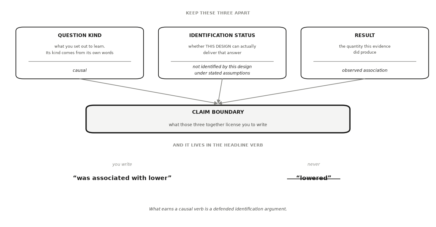
One more idea makes the claim’s honesty visible. Uncertainty in the same eye-span means the interval or caveat sits right beside the claim, not in a footnote (Wasserstein and Lazar 2016). Example: “about 6 points lower (95% interval: 1 to 11)” printed under the headline, so a reader meets the doubt at the same moment as the number. The numbers in this chapter’s examples are constructed to make the point; the uncertainty lesson you already worked through builds intervals properly. A bound a reader has to hunt for is a bound doing hidden work.
One more habit backs all of this. Traceability means every number you show walks back to the exact notebook cell that produced it. Example: the 6-point gap on your board points to the one line of code that computed it, and you can show that line when a judge asks. A number you cannot trace cannot go up.
28.3 A worked example
A biology student runs a small human-physiology pilot. Forty volunteers wear a step tracker for a month. Twenty walk at least 8,000 steps a day; twenty do not. Their average resting systolic blood pressure comes out at 128 in the active group and 134 in the less-active group, a 6-point gap.
The result is that 6-point gap. The claim is the decision. The draft headline reads “Walking LOWERS blood pressure,” drawn as two bars on an axis that starts at 125, which makes the small gap look like a cliff, with the two groups told apart by red and green alone.
Walk the decision. The question behind this study is causal, and it stays causal: you want to know whether walking lowers blood pressure. What the design cannot do is answer it. Nobody was assigned to walk, so the active group may differ in age, diet, or baseline health, and the comparison leaves that untouched. Fill the card: question kind causal, identification status not identified by this design, result an observed association. Those three together fix what the claim may say. The verb “lowers” claims a crossing the design never paid for, and the honest verb is “was associated with lower.” The truncated axis is the next problem: bars encode magnitude, so starting them at 125 makes a 6-point gap look like a cliff. Start the bars at a meaningful zero, or better, plot the two group averages as points with their intervals on a blood-pressure scale a clinician would recognize. The interval reported here runs roughly 1 to 11 points (constructed for the example), wide enough that the honest headline must carry it in the same eye-span. And each bar gets a direct value label, so a color-blind or screen-reader reader receives the number, not just the hue.
The locked claim: “In this sample, more-active volunteers averaged about 6 points lower resting systolic blood pressure (95% interval: 1 to 11); this is an observed association, and this design does not identify whether walking caused the drop.” Same result, a claim that survives the judge.
What licenses a causal verb is the identification argument, not the size of the gap you observed (Hernán and Robins 2020).
The block below builds the forty volunteers and prints the gap along with one thing the poster never showed: how the two groups differ before you compare them.
import numpy as np, pandas as pd
SEED = 464
rng = np.random.default_rng(SEED)

# Forty volunteers who CHOSE how much they walk. Age drives both.
n = 40
age = np.r_[rng.normal(31, 7, 20), rng.normal(43, 7, 20)]   # active are younger
active = np.r_[np.ones(20, bool), np.zeros(20, bool)]
systolic = np.round(112 + 0.5 * age + rng.normal(0, 6, n))

gap = systolic[~active].mean() - systolic[active].mean()
print(f"active group mean systolic      : {systolic[active].mean():.0f}")
print(f"less-active group mean systolic : {systolic[~active].mean():.0f}")
print(f"observed gap                    : {gap:.0f} points")
print(f"mean age, active vs less-active : {age[active].mean():.0f} vs "
      f"{age[~active].mean():.0f}")
print("\nnobody was assigned to walk. the age line is one difference you can")
print("see; the design leaves every unseen one untouched, so the verb stays")
print("'is associated with'")
28.4 Who it works for and why
Suppose you later run the walking study properly. Two hundred adults enroll, a coin decides who joins a walking program, and everyone’s resting blood pressure is measured at the end. The coin gives you the identification argument the pilot lacked, so the overall headline may now carry a causal verb. The next question arrives fast: does it work for everyone, and how does it work? Those are two questions, and each has its own trap.
Effect heterogeneity is the idea that a treatment can change an outcome by different amounts for different kinds of people. Example: a walking program might lower blood pressure more in older adults, whose pressure starts higher, than in twenty-year-olds. A moderator is a trait, measured before treatment, that marks those groups, such as age, sex, or starting blood pressure. The same question turns up in every field. An economist asks whether a job-training program raises earnings more for workers without a degree; a plant biologist asks whether a fertilizer helps a crop more on poor soil.
Two rules keep a subgroup claim inside its evidence. The first is timing. A pre-specified moderator is one you named in your declared design, with the reason you expect it to matter, before any outcome was measured. Example: “we expect a larger effect among adults over 50, because their pressure starts higher.” Cut the sample twenty ways after the fact and, by chance alone, one slice will probably look special. That slice is a lead for your next study, labeled exploratory in this one. Naming moderators in advance does not cure the arithmetic by itself: declare twenty and the same luck is waiting in one of them. Keep the list short, report how many differences you examined, and read any single striking one against that count.
The second rule is to test the difference, not the two labels. A result is usually called statistically significant when its 95% interval leaves out zero. A common slip reads one subgroup’s estimate as “significant,” the other’s as “not significant,” and concludes that the program works for one group and fails for the other. Gelman and Stern showed why that reasoning breaks: the gap between a significant result and a non-significant one need not itself be significant, or even large (Gelman and Stern 2006). A claim that the effect differs is a claim about one number, the difference between the two subgroup effects, and that number needs its own interval.
The block below builds a trial where the truth is simple: walking lowers systolic pressure by exactly 5 points in younger and older adults alike. Watch what the two subgroup estimates suggest, then read the last line.
import numpy as np, pandas as pd
SEED = 464
rng = np.random.default_rng(SEED)

# A randomized walking program. 140 younger and 60 older adults.
# The TRUE effect is the SAME in both groups: 5 points lower systolic.
younger = np.r_[np.ones(140, bool), np.zeros(60, bool)]
walk = rng.permutation(np.r_[np.ones(100, bool), np.zeros(100, bool)])
systolic = 125 + 12 * ~younger - 5 * walk + rng.normal(0, 12, 200)

def gap(mask):
    a, b = systolic[mask & walk], systolic[mask & ~walk]
    est = a.mean() - b.mean()
    se = np.sqrt(a.var(ddof=1) / len(a) + b.var(ddof=1) / len(b))
    return est, se

for name, mask in [("younger", younger), ("older", ~younger)]:
    est, se = gap(mask)
    print(f"{name:<8} effect estimate : {est:+.1f}  (95% interval {est-1.96*se:+.1f} to {est+1.96*se:+.1f})")
(ey, sy), (eo, so) = gap(younger), gap(~younger)
d, sd = eo - ey, np.sqrt(sy**2 + so**2)
print(f"difference, older minus younger : {d:+.1f}  (95% interval {d-1.96*sd:+.1f} to {d+1.96*sd:+.1f})")
print("\nthe truth is the same 5 points in both groups. the older group only")
print("looks twice as helped; read the difference line before you say so")
Among younger adults, walkers ended about 4 points below non-walkers (95% interval: 0.2 to 8.0); among older adults, about 10 points below (95% interval: 4.0 to 16.6). A draft headline would say the program works more than twice as well after fifty. The difference line disagrees: about 6 points, with an interval running from 13.6 points more benefit for older adults to 1.2 points more for younger ones. That interval includes zero, and you built this world so that the true difference is exactly zero. Sixty older adults split across two arms is a small sample. The claim the evidence licenses is: “we found no clear evidence that the effect differs by age (estimated difference: about 6 points more benefit for older adults, 95% interval from 13.6 points more to 1.2 points less).” Read that interval in both directions. It leaves room for no difference, and it also leaves room for a large one, so it is not evidence that the effect is the same for everyone either. Even a clear difference would have a limit. The coin assigned walking, never age, so a subgroup gap tells you where the effect is larger without telling you that age is the reason. Older adults also differ in weight, medication, and starting pressure.
The why question asks about a mechanism, the chain of steps through which a treatment changes an outcome. Example: walking might lower blood pressure partly through weight loss and partly through changes in the blood vessels themselves. A mediator is a variable on that chain, measured after treatment, such as body weight at the end of the program. The tempting analysis measures weight and reports how much of the effect “goes through” it. Imai, Keele, Tingley, and Yamamoto show that this split rests on an assumption the data cannot test, which they call sequential ignorability, and that randomizing the treatment secures only its first half (Imai et al. 2011). The second half says that, among people with the same treatment and the same background traits, weight is as good as randomly assigned. Nobody randomized the weight loss, so anything that drives both weight and pressure, such as a change in diet during the program, contaminates the split, and that holds even when the program itself caused the diet change. Their answer is a sensitivity analysis that asks how large a violation would have to be to erase the estimated indirect effect. Bullock, Green, and Ha reach the same verdict for psychology experiments: learning about a mediator usually takes a program of experiments built for that purpose (Bullock et al. 2010). The defensible default is to report the overall effect with its causal verb, and the program’s effect on weight with one too, since the coin assigned that comparison as well (“walkers ended the program lighter than the comparison group”). What the coin never assigned is weight itself, so the link from weight to pressure, and the share of the effect that runs through it, becomes a hypothesis your next design could test. Each of those sentences fills the same four-field card you used above; the mechanism sentence carries a status of not identified by this design.
A tool does the arithmetic here well. It will fit a model that lets the effect differ by group, compute the interval for a difference, and list moderators that other studies examined (each one a claim you check in the source). Its failure is just as predictable. Ask “who does the program work for?” and it will slice the data every way the columns allow, then return the slices that cleared a threshold, each with a fluent explanation attached. That is the twenty-slices trap run at machine speed. Your pre-specified list is the defense: the tool computes on the moderators you named, and anything else it finds goes under an exploratory label. Which moderators matter, and which mechanism you are willing to claim, stay your decisions.
When your question is how a process unfolds rather than how large an effect is, the qualitative inquiry route traces mechanisms through what people did and said, and the observational-causal pathway earlier in the book shows process tracing inside a single case.
28.5 Claims that travel
Now picture a second, larger walking trial: 400 volunteers on a campus, randomized the same way, and only about one in six of them over fifty. A public-health officer in a nearby retirement community reads your poster and asks the question every good result eventually meets: will this work for my residents? Your interval answers a question about the people you studied. Hers is about people you never enrolled. The number she wants is the average effect among her residents, a different estimand from the average effect among your volunteers. On the inquiry compass her question keeps its causal kind but moves its reach to a new setting, the cell the compass calls a transported effect. The coin licensed the causal claim for your volunteers; the crossing to her residents needs a license of its own, a transport argument, because random sampling from her community is one you do not have.
External validity is the extent to which a result from the people, treatment, outcome, and setting you studied holds for the ones someone else cares about. Findley, Kikuta, and Denly note that researchers invoke it constantly and rarely argue for it, and they recommend that studies report a routine discussion of it (Findley et al. 2021). Egami and Hartman split the question into four parts, one for each thing that can change between study and target: the population, the treatment, the outcome, and the context (Egami and Hartman 2023). Example, in your own trial: campus volunteers versus retirees (population), a supervised program versus a leaflet telling people to walk (treatment), pressure taken by a nurse versus a home cuff (outcome), and a walkable campus versus a suburb with no sidewalks (context). The other domains face the same four checks. A microfinance evaluation in one country, a get-out-the-vote experiment in one city, and a drought-tolerance result from a greenhouse all have to argue their way to the next country, city, or field.
Randomization does not settle any of this. It makes the comparison fair inside the trial, and that is all it promises. Deaton and Cartwright put it plainly: a trial’s estimate applies to the sample that was in it, and carrying it to any other group needs its own justification (Deaton and Cartwright 2018).
Two terms make that justification concrete. Your target population is the group you want your claim to speak about, named before you argue. Example: residents of one retirement community, most of them over seventy. Transport means carrying an estimate from the population you studied to a target population by reasoning about what differs between them. Moderators from the previous section whose mix differs between your sample and the target are what make transport hard. If the effect is larger for older adults, and the target is mostly older adults, the trial’s overall average is the wrong number for them.
When the difference that matters is one you measured, you can reweight. Reweighting means recomputing the average so each group counts in proportion to its share of the target rather than its share of your sample. Example: if older adults are 17 percent of your volunteers but 70 percent of the residents, the older adults’ effect gets a weight of 0.7. The block below builds a trial where the effect really does depend on age (3 points for younger adults, 9 for older ones), then recomputes the average as if seventy percent of the volunteers had been older, which is the target’s age mix.
import numpy as np, pandas as pd
SEED = 464
rng = np.random.default_rng(SEED)

# A randomized walking trial run on a campus: about 80% younger adults.
# In this constructed world the TRUE effect differs by age:
# 3 points lower for younger adults, 9 points lower for older adults.
n = 400
older = rng.random(n) < 0.20
walk = rng.permutation(np.r_[np.ones(n // 2, bool), np.zeros(n // 2, bool)])
systolic = 122 + 14 * older - np.where(older, 9, 3) * walk + rng.normal(0, 12, n)
df = pd.DataFrame({"older": older, "walk": walk, "sbp": systolic})

def effect(d):
    a, b = d.sbp[d.walk], d.sbp[~d.walk]
    return a.mean() - b.mean(), a.var(ddof=1) / len(a) + b.var(ddof=1) / len(b)

(e_all, v_all) = effect(df)
(e_y, v_y), (e_o, v_o) = effect(df[~df.older]), effect(df[df.older])
share_old = 0.70          # the retirement community you want to speak about
e_t = (1 - share_old) * e_y + share_old * e_o
se_t = np.sqrt((1 - share_old) ** 2 * v_y + share_old ** 2 * v_o)
print(f"older adults in the trial         : {older.mean():.0%}")
print(f"trial average effect              : {e_all:+.1f}  (95% interval {e_all-1.96*np.sqrt(v_all):+.1f} to {e_all+1.96*np.sqrt(v_all):+.1f})")
print(f"reweighted to a 70%-older target  : {e_t:+.1f}  (95% interval {e_t-1.96*se_t:+.1f} to {e_t+1.96*se_t:+.1f})")
print(f"true effect in that target        : {-(0.3*3 + 0.7*9):+.1f}")
print("\nreweighting fixes the age mix you measured. it cannot fix a")
print("difference between campus and community that you never measured")
Seventeen percent of the volunteers were older, and the trial’s average effect is about 2.8 points lower (95% interval: 0.4 to 5.3). Reweighted to the community’s age mix, the estimate becomes about 5.1 points lower (95% interval: 0.8 to 9.5), closer to the 7.2 points you planted for that target. Notice the price. The interval grew from about 5 points wide to about 9, because the transported number leans hard on the roughly seventy older volunteers. And the interval still treats the target’s 70 percent as known exactly. The whole calculation also rests on two assumptions. First, among people in the same age group, the effect on campus equals the effect in the community, so any other trait that changes the effect must be spread the same way in both places. Second, the trial held enough people of every kind the target contains to learn their effect at all. The first assumption hides a further one. Your “older” volunteers on a campus are likely in their fifties and sixties, and the residents are mostly past seventy, so the calculation also assumes a volunteer of fifty-five stands in for a resident of seventy-five. If the retirees also take blood-pressure medication or live without sidewalks, no reweighting of age repairs that. You argue it from what is known about those differences, or you narrow the claim.
That narrowing has a home on the card. Add a scope line under the claim boundary: “Scope: adults like these volunteers, in a setting like this campus; transport to older or less mobile groups assumes that, within an age group, nothing that changes the effect differs between campus and community.” A reader can now see where your claim stops traveling, instead of discovering it later.
AI tools generalize by default. Ask one to summarize your trial and it writes “walking lowers blood pressure in adults,” dropping the campus, the age mix, and the supervised program in one fluent sentence. That is a silent scope change aimed at the population rather than the verb. A tool is useful on the other side of the problem: it can list ways a target setting might differ from yours and draft the reweighting code. Each difference it lists is a claim to check against a real source, and choosing the target, and judging whether the unmeasured differences are small enough to defend, stays with you.
When several studies of the same question exist in different places, comparing their results is some of the most direct evidence you will get about whether an effect travels, though studies run in different places usually differ in design too. The evidence synthesis route shows how to gather those studies and read how much they disagree.
28.6 An AI failure case
You paste your honest headline into a tool and ask it to make it “punchier.” It returns, with total confidence, “Walking Reduces Blood Pressure by 6 Points.” It reads beautifully and it is wrong. The tool upgraded your verb from an association to a cause and dropped your interval, a silent scope change dressed up as a copy edit.
You catch it by comparing the new verb to what your design earned. Your question was causal and stays causal, but nobody was assigned to walk, so nothing identifies that answer and “reduces” claims a warrant you never held. You also notice the “6 points” now stands alone with no interval beside it. You revert to “was associated with about 6 points lower (95% interval: 1 to 11).” The fluent rewrite reviewed your style; only you can review your claim.
28.7 It is your turn
You are working inside Studio 9: Write, bound, and disclose. Keep what you write here; the studio’s milestone chapter is where it joins the other lessons’ pieces into one artifact you can defend.
After the last chapter you know where your confidence actually stops; this step turns each of your results into a sentence you would print and defend.
The hands-on half of this section lives in the chapter’s companion notebook: open it in Colab with the badge at the top, and work the steps there.
Commit your own answer first, then delegate. Each prompt is a checkable job, never a request for a verdict.
Expect to run each one more than once. You read what comes back, name the part that is wrong, and ask again with that correction in the prompt. That back-and-forth is the method, not a sign you prompted badly. Some tools now run several rounds on their own before showing you anything, which raises the stakes on your last step rather than lowering them, because more of the reasoning happened where you could not watch it.
Three calls stay yours. You choose the verb in your headline, the one word that fixes your claim boundary. You make the defend-or-concede call when a question pushes on that boundary out loud. And you make the lock decision: the judgment that every number is traced, every citation resolves, and the claim is ready to be final. A tool can draft questions and hunt sources, but it cannot decide what your evidence licenses or when your claim is earned.
List every result you might put in front of a reader, then write the claim sentence each one licenses.
Check every verb against what your design established, and downgrade the ones that reach too far. “Caused” becomes “was associated with”; “predicts” becomes “flagged.”
Red-team the verb.
Here is my written headline: "[paste it]." Act as a hostile reviewer and find every
place the verb claims more than an observational design licenses. Do not rewrite it
for me; list the exact words so I can fix them myself.
After running, verify: read each flagged word against your compass position and keep only the objections your design actually forces. Counters silent scope change (a claim quietly upgraded from association to cause).
Write a boundary line beside each claim naming what it does not establish, and put the uncertainty in the same eye-span as the number.
Turn your result into a checklist of hard questions.
Here is my headline claim: "[paste it]". My question is causal, my design is
observational and does not identify it, and what I actually estimated is a
descriptive association. Generate the eight hardest questions a skeptic would ask,
and mark which single audit each one belongs to: claim boundary, figure honesty,
uncertainty, or accessibility.
After running, verify: map every question to an audit and check it against your printed numbers; a missing audit is a gap the tidy list hid. Counters illusion of completeness (a long, organized list that skips the one flaw that matters most).
Trace every number back to the cell that produced it and cut the ones you cannot walk back. Then pick your lead claim, the sentence you would say first if you had ten seconds.
Log it in your AI Research Ledger, and verify at least one claim with a named method from the Verification Guide. An AI reviewer may run the check with you; the decision to accept or reject stays yours.
Locate the real source behind a physiology claim.
Act as a literature assistant in human physiology. My headline claims regular
walking is linked to lower blood pressure. Name up to three peer-reviewed sources
or clinical guidelines that support this, with title, authors, year, and venue.
Only list work you are confident exists; mark anything uncertain.
After running, verify: open each source in a library database and confirm it exists and says what you claim. Counters confident fabrication (an invented citation arrives as confidently as a real one).