43 Audit Studies: Testing How Institutions and AI Systems Treat Cases
This chapter is part of a book in active development and has not yet been through the author’s review. Content may change as the review advances.

The research decision. Decide which single attribute you will vary between otherwise identical cases, what response you will count, and whose time and consent your design uses to get it. No tool can make those choices for you, because each one fixes what your number describes and who pays for it.
43.1 Why this decision matters
The decision on the table: which one thing differs between your cases, and what your difference in responses is allowed to say.
“You sent the same résumé under two names and one name got more calls. Fine. Now tell me what the name told the employer. Was it race, or class, or a region, or all three? Tell me which employers you wrote to, and when. And tell me why you counted each email as a case when forty of them landed on the same desk.” — a labor economist, refereeing a correspondence study of hiring
An audit study looks simple, and that is its trap. You build two cases that differ in one attribute, send them out, and count replies. The count arrives quickly and looks decisive. But the attribute you varied may carry several signals at once. The replies may come from a handful of decision makers counted many times over. And the people who answered never agreed to take part. Get these wrong and a clean-looking gap describes something other than what your headline says, with more confidence than your data hold. This chapter gives you the decisions that make an audit’s number mean what you claim, whether the decision maker is a person or an AI system.
43.2 The concept
This chapter follows the audit-experiment design in the experimental-descriptive section of the RDSS design library (Blair et al. 2023). RDSS files the audit there on purpose. The coin flip decides which version of a case a decision maker sees, but the question RDSS asks is descriptive: how many decision makers in the sample treat the two versions differently. Randomization works here as a measuring instrument. RDSS also grants that the same randomized contrast can be read causally, as the average effect of sending one version instead of the other, and that this reading is correct. So place your question on the inquiry compass, not your instrument. “How many of these employers treat the two names differently?” is descriptive. “Does a name that signals this group change the callback rate?” is causal, and the random assignment of the version is what licenses that answer for the cases you sent. Either way, the reach is set by how you chose the decision makers. Drawn from a defined list, your answer can reach that list. Taken as whoever was convenient, it stays with the ones you wrote to, and you say so.
An audit study is a design that sends matched cases, identical except for one attribute you choose, to real decision makers and records how each case is treated. Example: two testers with the same scripted qualifications apply in person for the same jobs, and only one of them reports a criminal record (Pager 2003).
A correspondence study is an audit carried out entirely on paper or online, with fictitious applications instead of trained testers. Example: fictitious résumés sent in response to help-wanted ads in Boston and Chicago newspapers, with names chosen to sound White or Black, where the White-sounding names received about 50 percent more callbacks (Bertrand and Mullainathan 2004). Correspondence studies are cheaper and remove the tester’s behaviour from the comparison, which is one reason they are now common.
You can deliver the two versions in two ways. Matched pairs means each decision maker receives both versions, in randomized order. Example: every employer gets one application from each name set, a few days apart. Randomized single cases means each decision maker receives only one version, chosen by a coin flip. Example: each legislator gets one email asking for help, signed with a name chosen to sound Black or White (Butler and Broockman 2011). Pairs give more precision per decision maker. Single cases are harder for a decision maker to notice, because nobody sees two near-identical letters arrive in the same week.
Now the hard part. The signal problem is the fact that the attribute you vary usually carries more than one message. Example: a name can signal race and also social class, and names given mostly by more educated Black mothers are less often perceived as Black than names given by less educated mothers (Gaddis 2017). Your gap therefore measures the response to this name as read by these decision makers. Before you write “race,” you owe the reader evidence that the names signal race and little else. Pretesting how people perceive the names is the standard way to get it.
The estimand, the exact quantity your design is built to state, is narrow. It is the net response gap: the difference in response rates between the two versions, for these decision makers, these postings, and this period. Random assignment of the version is the warrant for it, and it needs nothing more. RDSS’s descriptive target is a different number: the share of decision makers who would respond to the first version but not to the second. The net gap equals that share only if almost nobody discriminates in the reverse direction. If some do, the net gap subtracts them from the others. It then understates the share who favour the first version, and it can sit near zero while many decision makers discriminate, in both directions (Blair et al. 2023). So report the net gap as what you measured. Write the word “share” only with that assumption stated beside it and defended for your decision makers. The warrant for extending the gap beyond the decision makers you reached is sampling. If you drew them from a defined list, such as every posting on a job board during one month, you may speak about that list. If you took whoever was convenient, you describe the ones you reached.
What the design cannot establish matters as much. An audit does not tell you why decision makers responded differently. Dislike of a group and a crude guess about productivity produce the same callback gap. It does not tell you what happens to wages or hires further down the line. It does not say how often real applicants face the gap either, because real applicants do not send identical résumés.
Two further terms protect the analysis. Clustering means that several responses come from the same decision maker or the same posting, so they rise and fall together instead of counting as separate cases. Example: forty applications sent to one national retailer may all be screened by the same recruiter under the same rule. Count the decision maker as the case, or compute an interval that allows for the grouping. Otherwise your interval will be too narrow. The post-treatment trap is comparing the quality of replies, such as tone or warmth, only among the decision makers who replied. Example: someone who never answers one name leaves no email whose tone you could score. So a tone comparison among repliers compares different kinds of people (Coppock 2019). Keep the response rate as your main outcome, and treat any quality measure as a separate analysis with its own assumptions.
43.3 Whose time, and whose consent
Audits of people carry an ethical cost that most designs do not. The decision makers did not agree to take part. The design only works if they do not know. You spend their time reading applications that do not exist. Any fictitious applicant who gets an invitation may hold an interview slot a real applicant needed, and a pair design doubles the letters each decision maker reads. That is why human audits need a formal determination before you send a single case. The ethics chapter walks you through the permission status. Expect a review board to ask you to justify waiving consent, to withdraw each fictitious application quickly once someone replies, and to say whether and how you will debrief the people you wrote to.
For a project that has one term to run, the realistic human route is reanalysis. Some published audits have released their data, and a careful replication or a new question asked of an existing audit dataset is a real contribution that needs no deception at all. If you still want to collect, the route in the rest of this chapter sits entirely outside human subjects: auditing an AI system.
43.4 Auditing an AI system
The same logic now tests machines. An algorithm audit is an audit study whose decision maker is an automated system, observed from the outside by feeding it controlled inputs and recording what it returns (Metaxa et al. 2021). Example: researchers created fake accounts that differed only in browser, operating system, or shopping history, ran the same searches on e-commerce sites, and recorded where prices and product rankings differed. They also had to separate those differences from ordinary noise such as inventory changes (Hannak et al. 2014). Another example comes from facial analysis. Commercial gender classifiers misclassified darker-skinned women far more often than lighter-skinned men (Buolamwini and Gebru 2018). Researchers have also varied the names inside prompts to a language model and found that its advice shifted with the name (Salinas et al. 2024). That study is a preprint, so read it as a design example, not a settled result. In biology, you could audit a plant-identification app by photographing the same specimens under randomized lighting and backgrounds and recording which conditions make it fail.
An AI audit of a tool you query yourself deceives no person, but it still has rules and traps. Read the tool’s terms of use before you send a single call, and never feed test cases into a live system where they land in a real person’s queue, such as an employer’s actual applicant pipeline. An AI partner is genuinely useful for the mechanical half: generating many template variants, running calls on a schedule, and logging every output with its build string. The traps below are where it needs you.
- Frozen configuration is the practice of recording the model’s exact version, the date, and every setting before the first call, and keeping them fixed for the whole run. Example: the vendor’s build string copied from the settings page, the temperature, and the system instructions, saved in your run record. A model can be updated overnight without notice. An audit that spans an update has measured two systems and blended them. That silent change is called drift.
- Temperature is the setting that controls how much a model’s output varies when you send the identical input again. Example: at a low temperature the same résumé gets nearly the same score every time; at a high one the score wanders.
- Nested outputs means that repeated outputs for the same prompt all come from one case. They still answer a question, only a narrow one. Example: fifty runs of one résumé under each name, on one frozen build, estimate how that build treats that résumé. For that estimand each run is a fair draw, and the run is the unit. They tell you almost nothing about the other résumés the model will meet. For a claim about how the screener treats résumés, the case is the template, exactly as the decision maker is the case in a human audit. Write down which of the two questions you are asking before you choose the unit. At a temperature of zero, repeats may return nearly the same output and add little even to the narrow question.
- A scoring rule is the written definition of what counts as a favourable response, fixed by you before you see any output. Example: “advance means a score of 7 or more out of 10,” or “the reply recommends an interview.” If you let another model judge the outputs, that evaluator model is a second instrument with its own errors. It is not ground truth. Check it against your own reading of a random subset before you trust its labels.
43.5 A worked example
Bring this into a business setting. A small firm is deciding whether to adopt an AI résumé screener. Before it does, you audit the screener. You write 60 résumé templates spanning the firm’s usual applicants. Each template is sent twice, once under a name drawn at random from set A and once under a name from set B. The two sets were pretested so that readers perceive them as differing in one group signal and not in class. Order is randomized, so neither name set always goes first, and any slow change in the tool over the afternoon cannot line up with one name set. The run record is written before the first call: build string, date, temperature, and the scoring rule. Everything is run in one afternoon.
This is the matched-pair logic of the classic correspondence study, moved from employers to software (Bertrand and Mullainathan 2004). The template is the case. The estimand is the difference in advance rates between the name sets, for this screener build, these name sets, these 60 templates, and these settings.
The block below uses a constructed screener in which a set-B name costs half a point on average. Watch the table of pairs: only the templates where the two names split carry information about the gap.
import numpy as np, pandas as pd
SEED = 464
rng = np.random.default_rng(SEED)

# Written BEFORE the first call, and never edited afterward.
run_record = {"tool": "resume screener, build string copied from its settings page",
              "date": "one afternoon, all calls", "temperature": 0,
              "rule": "advance = score of 7 or more out of 10"}

n = 60                                           # résumé templates = the cases
quality = rng.uniform(4, 9, n)                   # how strong each résumé reads
sent_first = np.where(rng.random(n) < 0.5, "set A", "set B")  # order, randomized
# CONSTRUCTED screener: a name from set B costs half a point on average.
score_a = np.clip(np.round(quality + rng.normal(0, 1.0, n)), 0, 10)
score_b = np.clip(np.round(quality - 0.5 + rng.normal(0, 1.0, n)), 0, 10)
adv_a, adv_b = score_a >= 7, score_b >= 7        # the rule, fixed in advance

pairs = pd.crosstab(pd.Series(adv_a, name="set A advanced"),
                    pd.Series(adv_b, name="set B advanced"))
print(f"set A name sent first : {np.mean(sent_first == 'set A')*100:.0f}% of templates")
print(pairs, "\n")
d = adv_a.astype(float) - adv_b                  # one difference per template
gap, se = d.mean(), d.std(ddof=1) / np.sqrt(n)
print(f"advance rate, set A names : {adv_a.mean()*100:.0f}%")
print(f"advance rate, set B names : {adv_b.mean()*100:.0f}%")
print(f"name gap                  : {gap*100:+.1f} points")
print(f"95% interval (templates)  : {(gap-1.96*se)*100:+.1f} to {(gap+1.96*se)*100:+.1f}")
print("\nonly the templates where the two names split carry the gap;")
print("this describes THIS tool, THIS build, THESE résumés")
Read the output as a referee would. Set-A names advanced on 62 percent of templates and set-B names on 48 percent. Most templates did not split at all: both names advanced on 28 and neither on 22. The gap comes from 10 templates, 9 where only the set-A name advanced and 1 where only the set-B name did. That net 8 templates out of 60 is the gap of 13.3 points, with a 95 percent interval from 3.5 to 23.2. Do not read the 9 as a count of templates the screener treats unfairly. In this constructed screener every template pays the same half point on average, and ordinary score noise alone makes pairs split in both directions. The net difference is the gap; the split counts are not a head count of penalised cases. The interval is wide because 60 templates are not many, and each template counts once. It also treats your 60 templates as a draw from the kinds of résumés the firm receives. You earn that reading by how you built them. Templates adapted from a random sample of the firm’s past applications, with personal details removed, earn it better than 60 résumés you invented at your desk.
The sentence you may write: “On 60 templates, this screener build advanced set-A names on about 13 more templates in every 100 than set-B names (95 percent interval roughly 4 to 23), under the settings in our run record.” The sentences you may not write are about every build of the tool, about the firm’s real applicant pool, or about the screener’s intent. The constructed half-point penalty is also an idea of the example. In a real audit you do not know the truth, which is the reason for the interval.
43.6 A seeded simulation
Two claims from this chapter can be checked by simulation. The first: an audit’s interval shrinks only as the number of cases grows. The second: repeating the same prompt many times does not add cases for a question about résumés in general, and treating those repeats as cases produces an interval that looks precise and misses that target. The code below builds a screener whose true name gap is 6 points on average across résumés. Some résumés trigger a large gap, some almost none, and about four in ten lean toward the other name. So the 6 points is a net gap. Reading it as the share of résumés the screener penalises would be wrong here, because the reverse cases pull it down. The seed makes the run reproduce exactly.
import numpy as np
import matplotlib.pyplot as plt

SEED = 464
rng = np.random.default_rng(SEED)
TRUE_GAP = 0.06                                   # 6 points, by construction

def templates(n):
    base = rng.uniform(0.40, 0.60, n)             # advance rate with a set-A name
    gap = rng.uniform(-0.24, 0.36, n)             # the name gap differs by résumé
    return base, base - gap                       # rates for set A, set B

# Left: one run per name per template, audits of growing size.
sizes, est, half = [10, 20, 40, 80, 160, 320], [], []
for n in sizes:
    pa, pb = templates(n)
    d = (rng.random(n) < pa).astype(float) - (rng.random(n) < pb)
    est.append(100 * d.mean())
    half.append(100 * 1.96 * d.std(ddof=1) / np.sqrt(n))
    print(f"{n:>3} templates: gap {est[-1]:+6.1f}, 95% interval "
          f"{est[-1]-half[-1]:+6.1f} to {est[-1]+half[-1]:+6.1f}")

# Right: 10 templates x 50 repeated runs per name = 1,000 outputs, rerun 1,000 times.
J, K, T_9 = 10, 50, 2.262                         # T_9: t value for 9 df
hits_naive = hits_clust = 0
for r in range(1000):
    pa, pb = templates(J)
    ya = rng.random((J, K)) < pa[:, None]
    yb = rng.random((J, K)) < pb[:, None]
    gap = ya.mean() - yb.mean()
    se_naive = np.sqrt((ya.mean()*(1-ya.mean()) + yb.mean()*(1-yb.mean())) / (J*K))
    se_clust = (ya.mean(axis=1) - yb.mean(axis=1)).std(ddof=1) / np.sqrt(J)
    hits_naive += abs(gap - TRUE_GAP) <= 1.96 * se_naive
    hits_clust += abs(gap - TRUE_GAP) <= T_9 * se_clust
    if r == 0:                                    # keep the first audit to plot
        g0 = 100 * gap
        ci = {"naive": (g0 - 196*se_naive, g0 + 196*se_naive),
              "clustered": (g0 - 100*T_9*se_clust, g0 + 100*T_9*se_clust)}
print(f"\nfirst audit, gap {g0:+.1f}")
for k, (lo, hi) in ci.items():
    print(f"  {k:9s} interval : {lo:+.1f} to {hi:+.1f}")
print(f"\nnaive intervals cover the truth     : {hits_naive/10:.0f}% of reruns")
print(f"clustered intervals cover the truth : {hits_clust/10:.0f}% of reruns")

fig, (a1, a2) = plt.subplots(1, 2, figsize=(9.6, 3.6))
a1.errorbar(range(6), est, yerr=half, fmt="o", color="#2a78d6", capsize=3)
a1.axhline(100 * TRUE_GAP, color="#333333", ls="--")
a1.set_xticks(range(6), sizes)
a1.set_xlabel("Résumé templates in the audit (one run per name)")
a1.set_ylabel("Name gap in advance rate (points)")
for y, (k, col) in enumerate([("clustered", "#2a78d6"), ("naive", "#eb6834")]):
    a2.plot(ci[k], [y, y], color=col, lw=3)
    a2.plot([g0], [y], "o", color=col)
a2.axvline(100 * TRUE_GAP, color="#333333", ls="--")
a2.axvline(0, color="#999999", lw=.8)
a2.set_yticks([0, 1], ["clustered", "naive"])
a2.set_xlabel("Name gap in advance rate (points)")
plt.show()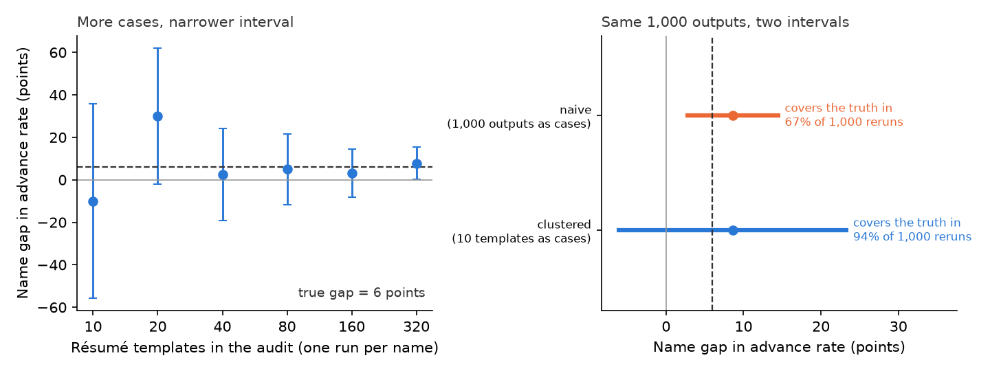
Read the left panel first. With 10 templates, the estimate came out at minus 10.0 points, pointing the wrong way, with an interval from minus 55.7 to plus 35.7. That interval is honest: 10 cases cannot tell a large gap from none. With 320 templates the estimate is 7.8 and the interval runs from plus 0.2 to plus 15.5, close to the true 6 and narrow enough to say something. The estimates wander on the way, and at 20 templates one run landed at plus 30.0. Each audit is a single draw, which is why the interval travels with the estimate every time.
Now the right panel. The same 1,000 outputs, 10 templates run 50 times per name, give one estimate of 8.6 points and two intervals. The naive interval treats every output as a new case and runs from 2.5 to 14.7. It excludes zero and looks like a finding. The clustered interval treats each template as one case and runs from minus 6.4 to 23.6, which is what 10 cases can actually support. The true gap here is the average over all the résumés the screener might meet, so the number of templates, not the number of outputs, sets the precision. Across 1,000 reruns of the whole audit, the naive interval covered the true gap only 67 percent of the time, against a promised 95. The clustered interval covered it 94 percent of the time. The naive interval is not wrong about everything. For a narrower target, the average gap on these 10 templates alone, its width is about right. It fails because the question was about résumés the audit never sent. Repeating a prompt measures how that prompt fares. It does not tell you how the model treats résumés you did not send. In the companion notebook, change J, K, T_9 to 40, 12, 2.023 (2.023 is the t value for 39 degrees of freedom). The audit then spends about the same budget on more templates. Watch the two intervals move closer together and the naive coverage climb toward the clustered one.
43.7 An AI failure case
You ask an agentic tool to run your screener audit. You give it one résumé template and two name sets, and it comes back with a tidy report. “I ran the prompt 50 times for each name (n = 50 per group). Set-A names advanced in 41 of 50 runs, set-B names in 29 of 50, a statistically significant difference of 24 points.” The code ran, the numbers add up, and the table is clean.
This is two named failures. It is plausible-but-wrong-method, because the report treats 100 draws from one case as if they were 100 independent résumés. The test itself answers a real but narrow question: on one frozen build, does this one template advance more often under one name set? For that estimand, 50 runs per name are fair draws. It is also silent scope change, because a statement about one résumé became a finding about the screener. The arithmetic is fine; the unit is wrong for the claim. For any claim about the screener’s treatment of résumés, the audit has one case, and the right sample size is 1. Read its log closely and a third problem appears, and it breaks even the narrow reading. Halfway through the run, the tool’s calls started returning a different build string. The vendor had pushed an update, so the 50 runs per name straddle two systems and are not draws from one set of outputs.
A tidy count is not a sample. You catch it by asking the question the report skipped: what is the case here, and how many of them are there? Then you check the build string on every output line against your run record. Rewrite the result as what it is: “For one template, under builds X and Y, set-A names advanced more often,” and split the runs by build before you test even that. Then rerun the audit with many templates on one frozen build, and log why.
43.8 It is your turn
A further route beyond the five pathways. This lesson extends Studio 5: Develop the pathway. Read it once you have declared your primary pathway and your question calls for this design. Studio 5’s milestone asks for the same decisions, answered for this route.
Your design is declared and diagnosed. This route asks you to name the one attribute you will vary, the case your number is about, and whose time the design spends.
The hands-on half of this section lives in the chapter’s companion notebook: open it in Colab with the badge at the top, and work the steps there.
Commit your own answer first, then delegate. Each prompt below is a checkable job, not a request for a verdict. Work them as a loop. The first answer is a draft: find the claim you cannot check, say so in your next message, and run it again. Some tools will run a whole audit unattended and hand you a finished report. That is exactly when you check what the case was and which build answered.
Three calls stay yours. You decide which attribute you vary and what it signals, because the meaning of a name or a photo is a judgment about how decision makers read it. You decide what counts as a favourable response, and you write that scoring rule before you see a single output. And you decide whether this audit may be run at all: whose time it spends, whether it deceives anyone, and what permission it needs. A tool can draft cases, run calls, and tabulate replies. You own the claim, its unit, and its boundary.
Write your audit question as one sentence naming the decision maker, the attribute, and the response. Underneath it, write the estimand: the net difference in response rates, for which decision makers or which system build, over which cases and which period. Say whether the question is descriptive (how many treat the versions differently) or causal (what sending one version instead of the other does).
Name the attribute’s signals. List everything your chosen names, photos, or phrases might tell a reader besides the one attribute you intend. Then say how you will check what they actually signal.
Commit your own list before you delegate.
When you are ready to delegate this step:
I plan an audit that varies [attribute] using these versions: [paste your
names, photos, or phrases]. Act as a skeptical sociologist. List every
attribute a reader might infer from each version besides the one I intend,
in a table with the version, the extra signal, and which direction it could
push my response gap. Do not suggest replacement versions; I will choose them.
After running, verify: compare the table with the list you wrote first, and look for a published pretest of how people perceive your versions before you trust either list. Counters illusion of completeness (a tidy table that omits the one signal your reader will raise first).
Declare your case and your data strategy. Say what one case is (a decision maker, a posting, a template), how many you will have, how they were chosen, and whether each case gets both versions or one. If you plan repeated runs of one prompt, say whether they serve a claim about that prompt or only steady its score. If you are auditing an AI system, write the run record now: build string, date, every setting, and the scoring rule.
Declare your answer strategy and its warrant. State the comparison you will compute, which is the net gap, and the interval you will attach to it with the case as the unit. If you also want to call the gap a share of decision makers who discriminate, state the assumption that reading needs (almost no one favours the other version) and why it is plausible for your decision makers; if you cannot defend it, report the net gap alone. Then say which population, if any, your sampling lets you speak about, and write one sentence on what the audit cannot establish: why the decision makers responded as they did, or what real applicants face.
When you are ready to delegate this step:
Here is my audit plan: [paste steps 1 to 4]. Act as a hostile referee of
audit studies. Tell me where my responses are not independent cases for the
claim I state: the same decision maker, the same posting, the same prompt,
or the same model build. For each, say what the true number of cases is.
Do not rewrite the plan for me.
After running, verify: count your cases by hand from your own plan and compare the number with the referee’s. If it only praises the plan, push back with “assume my interval is too narrow; name the reason.” Counters sycophantic agreement (praise that reviews your ego, not your evidence).
Settle the permission question. If real people receive your cases, write your permission status and the competent authority you will ask. Then write the no-deception route you will take if the answer is no: reanalysis of a published audit’s open data, or an audit of an AI system.
When you are ready to delegate this step:
Act as a research librarian in economics and political science. Find
published correspondence or audit studies whose authors released their
response-level data. For each give authors, year, venue, the attribute
varied, and where the data are archived. Only include work you are
confident exists; mark anything uncertain.
After running, verify: open each archive yourself and download the file before you cite it; treat any study or dataset you cannot find as a possible confident fabrication and leave it out.
Log the step in your AI Research Ledger, and verify at least one output with a named method from the Verification Guide. A benchmark result is the natural check for an audit’s pipeline: run it on a published audit’s open data, or on the worked example above, and confirm it reproduces the reported gap and interval within rounding. A falsification test is the strong second check. Send a slice of cases where both versions carry the same name. If your setup is sound, that gap should sit near zero within its interval; a clear gap there means something besides the name differs, such as order or a changed build. A gap near zero is reassuring; it does not show the pipeline is flawless. An AI reviewer may run the checks with you; the decision to accept or reject stays yours.