17 Prediction and Generalization
This chapter is part of a book in active development and has not yet been through the author’s review. Content may change as the review advances.

The research decision. Decide whether your question is truly a forecast about cases nobody has seen yet, and if it is, sign a four-part contract before you fit anything: target, baseline, split, metric, plus a leakage check. That contract is what lets you defend a modest honest score and say out loud where your forecast stops working.
17.1 Why this decision matters
The decision on the table: whether you are forecasting unseen cases, and if you are, what score you would accept as honest.
Picture a county public-health officer who must decide, week by week, whether to post a swimming advisory at a lake. Blooms of cyanobacteria can turn a safe beach into a health hazard within days. A vendor arrives with a model that flags harmful blooms “with 94% accuracy.”
“Ninety-four percent compared to WHAT? Most weeks this lake is fine, so if I just say ‘no bloom’ every single week I am already right about eighty-five percent of the time. If your model cannot clearly beat that, and prove it did so on weeks it never studied, I am not closing a public beach on its say-so.” — a public-health officer who has been burned by an impressive-sounding number
That officer asks the two questions this chapter trains you to answer before you trust any forecast. Is it better than the dumbest honest rule, and was it earned on cases the model never saw? Get those wrong and you cry wolf or miss a real hazard.
17.2 The concept
This pathway is the book’s own addition. The four pathways around it adapt RDSS’s design library; prediction extends that library rather than adapting a part of it, because a forecast is judged by how it performs on cases nobody has seen yet (Blair et al. 2023).
A prediction is a best guess about a case whose outcome you cannot see yet. Example: forecasting whether a lake blooms next week, before next week exists. Prediction is descriptive, not causal. It forecasts what will happen, never why.
What makes prediction its own question is its reach, the cases a claim is meant to cover. Prediction’s reach is unseen cases, units not in your data whose outcome is still unknown, such as next month’s samples. Its cousin is generalization, reach from your sample to a broader population, such as from the twelve lakes you measured to every lake in the watershed. Both go beyond the data in hand, and both are honest only when you can name the crossing that licenses them.
A forecast earns trust under a four-part contract, in fixed order. The target is the one column you predict, for example bloom_next_week. The baseline is the dumbest honest rule you must beat, usually “always guess the most common answer”; if 85% of weeks have no bloom, that rule scores 85% for free, so 85% is the bar. The metric is how you keep score, matched to the target; accuracy misleads when blooms are rare, so recall on the bloom class, the share of real blooms the model catches, often matters more. Whichever you choose, score the baseline and every candidate on the same metric, or the comparison means nothing.
The split is where most honest-looking forecasts go wrong, so it gets three parts rather than two. The training set is the data each candidate model learns from. Example: the model works out its coefficients from your first summer. The selection set is separate data you use to choose among candidates. Example: you compare three feature lists and pick one on your second summer. The final holdout is data you lock away and open exactly once, after every choice is settled. Example: only the model you already chose ever touches your third summer.
Run them in that order. Fit on training, choose on selection, then score your one choice on the final holdout. The reason for the middle step is easy to miss. When you try twelve models and keep the best score you saw, that winning score is flattered by luck on average: some model was always going to look best on that particular data, partly because its errors happened to fall kindly there. On any one split the flattery can be large, small, or even reversed; over many splits it points up. Model-selection bias is that flattery, the gap between a winner’s score on the data that crowned it and its honest score on data it has never met (Varma and Simon 2006). Report the crowning score as final and you will promise performance the model cannot deliver.
One consequence is worth stating plainly. If the final holdout makes you go back and change a feature, a threshold, or a model, it has joined development and stopped being an exam. You then need fresh untouched data for the next final check. In the simple workflow this book teaches, seeing the final score seals the analysis; any change after it breaks the seal. Specialists have techniques for careful reuse, and they are beyond this chapter, so hold the simple rule until you have a defended reason not to.
One trap sits above all others. Data leakage is information reaching your model, or your choice of model, that would not be available at the real forecast moment (Kaufman et al. 2011). Example: the toxin concentration measured during the bloom. A leaked feature inflates your score on today’s data and collapses on tomorrow’s, because it will not exist when you truly need the forecast. Choosing your model on the final holdout is the same failure wearing different clothes, since that score was supposed to stand in for data you have never seen.
Time carries its own version of this trap. When your target is next week, your exam weeks should come after the weeks you learned from. Splitting weeks at random hands the model August while asking it to forecast July, which answers how well it fills in scattered past weeks rather than how well it forecasts the next one. Keep the blocks in calendar order, and let the latest block be the one you lock. That is the default that mimics how the forecast will actually be used; specialists relax it in narrow, argued cases, and none of them starts by shuffling the calendar.
17.3 A worked example
Suppose you want to warn swimmers a week ahead. Your target is bloom_next_week, one if the lake exceeds the advisory threshold and zero otherwise. Across three summers of weekly samples, 85% of weeks are clear, so your baseline, “always say no bloom,” scores 0.85 with no model at all.
You keep features genuinely known a week early: water temperature, recent rainfall, upstream phosphorus load. The three summers give you your three roles without any shuffling (Hastie et al. 2009). Summer one trains your candidate models. Summer two chooses between them. Summer three stays locked until the choice is made. You fit a logistic model (a standard yes-or-no classifier) and compare a few feature lists on summer two. Then you open summer three once, for the winner alone. Scored on the same metric as the baseline, accuracy, the model lands around 0.88 against the baseline’s 0.85 (these scores are constructed for the example). That three-point edge feels small, and its smallness is the honest result: a modest true win beats a dramatic fake one. You still report recall beside it, since accuracy alone hides the missed blooms.
Then a well-meaning collaborator adds chlorophyll_a, the pigment reading. The score leaps to 0.97. Exciting, until you ask when chlorophyll is measured: during the very bloom you are forecasting. It is the outcome wearing a different label. Drop it, and the score falls back to 0.88. The timing test, not the accuracy, decides. And because you trained on one shallow lake, you name the boundary out loud: on a deep, cold reservoir the pattern may not hold, so the forecast does not yet generalize there.
The block below builds the three summers, keeps the last one locked, and scores the honest model and the leaking one on the same rows. The scores are constructed for the example; the ordering is the lesson.
import numpy as np, pandas as pd
SEED = 464
rng = np.random.default_rng(SEED)

# 120 weekly samples across three summers, 40 weeks each, six bloom weeks per
# summer (15%). The calendar order is the design: it decides the three roles.
summer = np.repeat([1, 2, 3], 40)
bloom = np.zeros(120, dtype=bool)
for s in (1, 2, 3):
    weeks = np.where(summer == s)[0]
    bloom[rng.choice(weeks, 6, replace=False)] = True

temp = 22 + 3.0 * bloom + rng.normal(0, 2.0, size=120)     # known a week early
rain = 20 + 4.0 * bloom + rng.normal(0, 6.0, size=120)     # known a week early
chl = 5 + 30 * bloom + rng.normal(0, 8.0, size=120)        # measured DURING it

train, locked = summer == 1, summer == 3
z = lambda v: (v - v[train].mean()) / v[train].std()
acc = lambda pred: float((pred == bloom[locked]).mean())

baseline = acc(np.zeros(locked.sum(), dtype=bool))         # always "no bloom"
score = 0.55 * z(temp) + 0.35 * z(rain)
honest = acc(score[locked] > np.quantile(score[train], 0.85))
leaky = acc(chl[locked] > np.quantile(chl[train], 0.85))

print(f"baseline, always say 'no bloom' : {baseline:.2f}")
print(f"honest features, locked summer  : {honest:.2f}")
print(f"with chlorophyll_a added        : {leaky:.2f}")
print("\nthe third number is not skill. chlorophyll is measured during the")
print("bloom you claim to forecast, so it cannot exist at prediction time")
17.4 A seeded simulation
The chapter claims two things at once, and the code below shows both. A model can get better at data it has already seen while getting worse at cases it has never seen. And the score that crowned your winner flatters it on average. The seed makes the run reproducible: the same code always draws the same worlds.
The first half builds one world (a sine curve plus noise) and runs the protocol you just learned: twelve polynomials fit on training, compared on selection, and the winner alone scored once on a final holdout. The second half measures model-selection bias the way the definition demands, as an average over repetitions. In each of 500 fresh worlds it asks: how does the winner’s true error compare with the selection score that crowned it? Nobody can measure a model’s true error exactly, so the code stands in for it with ten thousand fresh points, which is close enough to trust and far more than any real study would have. Each half restarts the seed, so you can run either one on its own and get these same numbers.
import numpy as np

SEED = 464
degrees = np.arange(1, 13)

def world(rng, n):
    x = rng.uniform(-3, 3, n)
    return x, np.sin(1.5 * x) + rng.normal(0, .35, n)

def rmse(coefs, data):
    x, y = data
    return np.sqrt(np.mean((np.polyval(coefs, x) - y) ** 2))

# Left panel: one world, the three roles.
rng = np.random.default_rng(SEED)
training, selection, final = (world(rng, 40) for _ in range(3))
fits = [np.polyfit(training[0], training[1], d) for d in degrees]
sel_err = np.array([rmse(c, selection) for c in fits])
chosen = int(np.argmin(sel_err))          # chosen on SELECTION, never final
print("chosen degree:", degrees[chosen])
print("selection score that chose it:", round(float(sel_err[chosen]), 3))
print("its one final-holdout score:  ", round(rmse(fits[chosen], final), 3))

# Right panel: optimism in expectation. Restart the seed so this study
# reproduces on its own.
rng = np.random.default_rng(SEED)
gaps = []
for _ in range(500):
    tr, sel, big = world(rng, 40), world(rng, 40), world(rng, 10_000)
    f = [np.polyfit(tr[0], tr[1], d) for d in degrees]
    se = np.array([rmse(c, sel) for c in f])
    pick = int(np.argmin(se))
    gaps.append(rmse(f[pick], big) - se[pick])   # true error minus its crown
gaps = np.asarray(gaps)

print("mean optimism:", round(float(gaps.mean()), 3), "RMSE")
print("median:", round(float(np.median(gaps)), 3))
print("winner truly worse than its crowning score in",
      round(100 * float((gaps > 0).mean()), 1), "% of worlds")
print("largest single gap:", round(float(gaps.max()), 2))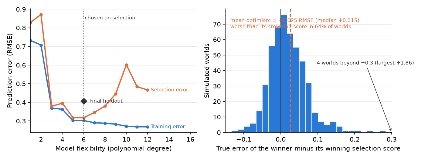
Read the left panel first. The blue training error only falls: every extra degree of flexibility lets the model bend closer to points it has already seen. The orange selection error falls while the model is learning signal, bottoms out near degree six, and climbs as the model starts memorizing noise. Nothing in the blue line alone would ever tell you to stop at six. Only data the fit never touched can say that.
Now the right panel, and read it as an average, because that is what the bias is. Across 500 worlds the winner’s true error exceeds the score that crowned it by 0.025 RMSE on average (median 0.015), and the winner comes out worse than its crowning score in 64 percent of worlds. In the other third, luck ran the other way, which is why no single split can show you the bias: it is a lean in the pile, not a property of each run.
Then look at the arrow. In 4 of the 500 worlds the gap blew past +0.3, topping out at +1.86, because a wildly flexible fit happened to win selection and then swung hard outside its data. Those worlds are not noise to trim away. They are the procedure’s real risk showing itself, and any average you report has to own them. The honest summary names all three things: the lean (the mean), the typical case (the median), and the tail (how bad, how often). In the companion notebook, rerun the simulation at several noise levels (the .35) and compare the mean, the median, the frequency, and the maximum separately. The average optimism grows with noise; a single seeded extreme, like this run’s +1.86, need not move the same way, because one world’s worst luck is not a summary of the procedure.
17.5 Forecasting over time: rolling-origin evaluation
The three summers in the worked example give your forecast one exam: learn from the past, then score once on what came next. A kayak-rental owner at the same lake needs more than one exam. At the end of every month she books staff for the month ahead, so she makes the same forecast twelve times a year, each time from a new starting point. She needs the method’s record across all of them.
The forecast origin is the last moment whose data you may use to make a forecast. Example: when she forecasts July at the end of June, June 30 is the origin, and nothing recorded after it may enter the forecast. The forecast horizon is how far past the origin the forecast reaches. Example: one month ahead for next month’s schedule, three months ahead if she must hire in April for July.
Rolling-origin evaluation is scoring a forecasting method by repeating the forecast from many origins in calendar order, each time using only the data before that origin and scoring the months after it (Tashman 2000). Example: forecast month 37 from months 1 to 36, then month 38 from months 1 to 37, keeping one error per origin. An expanding window is training data that grows by one period at each new origin. Example: the window starts with three years of history and ends with almost nine. A rolling window keeps a fixed length and drops its oldest month as each new one arrives. Example: always the latest five years, for a business whose distant past no longer resembles its present.
Seasonal data change what the dumbest honest baseline looks like. The seasonal naive forecast is a forecast equal to the value observed in the same season one cycle earlier (Hyndman and Athanasopoulos 2021). Example: this July’s rentals will equal last July’s. It costs nothing and already knows about summer, so a method that cannot beat it has added nothing, on this score, that last year’s ledger did not already say. Keep score with the mean absolute error, which is the average size of a miss, ignoring whether the forecast was too high or too low. Example: misses of 10 rentals over and 30 under average to 20.
The block below builds ten years of constructed monthly rentals whose business level drifts, and compares the seasonal naive forecast with a “seasonal step”: start from the latest month and add the usual change between that calendar month and the target month in earlier years. Origins whose target months fall in years four to nine compare the two; year ten stays locked, the way the third summer did. Every origin uses an expanding window: all the months before it, and nothing after.
import numpy as np
SEED = 464
rng = np.random.default_rng(SEED)

# Ten years (120 months) of kayak rentals at a lake: a summer peak plus a
# business level that WANDERS month to month. Constructed, not real data.
month = np.arange(120)
summer = 300 * np.sin(2 * np.pi * (month % 12 - 3) / 12).clip(0)
level = 250 + np.cumsum(rng.normal(0, 15, 120))
rentals = level + summer + rng.normal(0, 10, 120)

def errors(origin, h):
    """Forecast h months past the origin (the end of month origin-1),
    using months 0..origin-1 ONLY: an expanding window."""
    y, last, target = rentals[:origin], origin - 1, origin + h - 1
    naive = y[target - 12]                              # same month last year
    steps = [y[s + h] - y[s] for s in range(last % 12, last - h + 1, 12)]
    step = y[last] + np.mean(steps)    # latest month + its usual seasonal step
    return abs(rentals[target] - naive), abs(rentals[target] - step)

# Origins in years 4-9 compare the two methods; year 10 stays locked.
for h in (1, 3, 6):
    e = np.array([errors(o, h) for o in range(36, 108 - h + 1)])
    print(f"horizon {h}: {len(e)} origins | seasonal naive {e[:, 0].mean():4.1f}"
          f" | seasonal step {e[:, 1].mean():4.1f} | step closer at"
          f" {int((e[:, 1] < e[:, 0]).sum())}")
final = np.array([errors(o, 1) for o in range(108, 120)])
print(f"\nlocked year 10, horizon 1: naive {final[:, 0].mean():.1f}, "
      f"step {final[:, 1].mean():.1f}, step's single-month errors "
      f"{final[:, 1].min():.0f} to {final[:, 1].max():.0f}")
print("\nerrors are average misses in rentals; the baseline was closer at")
print("some single origins, so one origin alone can crown the wrong method")
One month ahead, across 72 origins, the seasonal step misses by 18.5 rentals on average against the baseline’s 43.9. The step’s average miss grows to 26.0 at three months and 34.4 at six. The baseline hardly moves (43.9 to 46.1), because at any horizon up to twelve months it forecasts a given month the same way, by copying that month a year earlier; its small drift reflects slightly different target months. The step wins by knowing the latest level, and that knowledge goes stale as the horizon stretches. So the verdict depends on the decision: the step earns its keep for next month’s schedule, and its edge narrows for April hiring.
Two readings keep the result bounded. The baseline was closer at 17 of the 72 one-month origins, so a single origin would have crowned the wrong method about one time in four. And those 72 errors are not 72 independent trials. Neighboring origins share almost all of their training months, and the misses they score build up over overlapping stretches of months. The step’s miss builds up over the months of its horizon; the baseline’s builds up over the whole year since the month it copies, even one month ahead. So one surprise in the business level spoils several errors in a row. A margin of error computed as if each origin were a fresh case would be too narrow. The locked year, opened once, agrees with the comparison: 18.5 for the step against 76.8 for the baseline, in a year when the business level moved a lot. Twelve locked months are thin evidence, and the step’s single-month errors ran from 1 to 58, so report that spread beside the average.
State what this licenses. The estimand here is the average size of a miss for a forecast made at a stated horizon, for months like the ones still to come. The warrant is the chapter’s crossing to unseen cases, applied at every origin: only information available at the origin enters the forecast, and each error is scored on a month the method had not seen. Compare many methods on the same origins and the winner’s average becomes a selection score with model-selection bias, which is why year ten stays locked. What rolling origins cannot establish is why rentals move, or how the method behaves after a break the history never showed, such as a rival opening across the lake.
Leakage in a time series often hides in preparation steps. A seasonal pattern or a scaling computed on the whole series before the loop begins lets every early forecast peek at later summers. In economics, many official series are revised after first release, so feeding a forecast today’s revised figures hands it numbers the forecaster at the origin never saw (Croushore and Stark 2001). Decide, too, which release you score the forecast against, the first one or the latest, and say so. The chapter’s timing test catches each of these, provided you ask it at each origin about the date each figure was released, not only the period it describes.
This is good work to hand an AI assistant. It writes a rolling-origin loop in seconds. It slips in two familiar places. It reaches for a library’s ordinary cross-validation, whose folds ignore the calendar and train on later months to forecast earlier ones, or it standardizes the data once, above the loop, using every month at once. Both return a flattering number. Read the loop for one thing: at each origin, does any line touch a row recorded after that origin? The horizon stays yours too, because it comes from the decision the forecast serves, which no tool knows.
A forecast from before a known start date can also stand in for what would have happened without a new policy. That question is causal rather than predictive, and it has its own route: interrupted time series, in Chapter 41.
17.6 An AI failure case
You paste your feature list and ask an AI partner which features are safe to use. It answers with confidence: “chlorophyll_a is your strongest predictor, keep it.” The reasoning sounds airtight, because chlorophyll correlates almost perfectly with blooms. That near-perfect correlation is exactly the tell. This is the plausible-but-wrong-method failure: the tool ranked the feature on how well it fits the past, not on whether it could exist in time for a forecast. You catch it with one question statistics alone cannot answer. When is chlorophyll measured? During the bloom, so no forecast made a week earlier could have it. Drop it, watch the score fall back to 0.88, and keep the honest model.
17.7 It is your turn
You are working inside Studio 5: Develop the pathway. This lesson serves the prediction pathway. If your declared pathway is different, skim it and work the lesson that matches; the studio page routes you.
Your design is declared and diagnosed. This step decides whether your project is really forecasting cases nobody has seen yet, and if it is, puts that forecast under contract before you fit a single model.
The hands-on half of this section lives in the chapter’s companion notebook: open it in Colab with the badge at the top, and work the steps there.
Commit your own answer first, then delegate. Paste real output, never a number you remember. Expect to run each prompt more than once: read the answer, name the part you do not believe, put that objection back into the prompt, run it again. Tools that run that loop by themselves, fitting and refitting a model across several turns, make the leakage question below more urgent rather than less. Nobody in the loop but you knows when your data were recorded.
Four calls stay yours. The target: what you forecast and why it matters. The baseline: the honest rule the model must beat. The timing of every feature: whether a value would truly exist at the forecast moment, which only you, who knows your data’s timeline, can settle. And the verdict on whether your project should predict at all. A tool that has never seen your timeline cannot make these calls for you.
Ask the blunt version of your question: does your project need to guess an outcome for a case whose outcome does not exist yet? Write yes or no, and the one sentence that justifies your answer.
If yes, sign the four-part contract, in order. Name the target column, the dumbest honest baseline it has to beat, the split, and the metric matched to how rare your outcome is. Give the split all three of its roles: which data fit your candidates, which data choose between them, and which data stay locked for the single final score. If your target is about a later time, order those three blocks by the calendar and lock the latest one.
When you are ready to delegate this step:
Act as a Python tutor. Here is my forecasting workflow: [paste the cells
that split, fit, compare, and score]. Audit the three data roles one by
one. Which rows fit the candidates? Which rows chose between them? Which
rows produced the final score, and had any model already seen them, even
indirectly through my choices? If my target is about a later time, check
whether every training row is earlier than the rows it is scored on.
Then give me one independent way to confirm the final rows never touched
training or selection.
After running, verify: read the baseline, model, and margin off your own printout and confirm the tool’s numbers match, not ones it guessed. If the audit finds a role missing, that is the finding; do not argue the score. Counters confident fabrication, a fluent walkthrough quoting a margin your code never produced.
List your features and write beside each one the moment its value is settled. Circle anything settled at or after the outcome. That circled set is your leakage list, and it belongs in your write-up whether or not you drop the features on it.
When you are ready to delegate this step:
Here is the outcome I want to predict and the moment I need the forecast:
a bloom next week, decided by next week's samples. Here is my candidate
feature list with when each value is recorded: [list]. For each feature,
say whether its value is settled before, at, or after the outcome, and
flag any that could not exist at prediction time.
After running, verify: re-derive the timing of the one feature it clears most confidently. If any feature is settled at or after the bloom, reject it whatever the tool says. Counters illusion of completeness, a tidy list omitting the one late-settled feature that dooms the forecast.
Write the boundary in one sentence: the cases your forecast covers, and the ones a reader should not assume it covers. Be specific about what makes them different.
When you are ready to delegate this step:
Act as a hostile reviewer. Attack this headline: "Our model forecasts
blooms with 88% held-out accuracy." Name every reason a skeptic would
distrust it, including the baseline it beat, the metric, and any hidden
leak.
After running, verify: check each objection against your printout and keep the ones your numbers support. Counters sycophantic agreement, where an assistant primed to help praises a headline you wrote.
If prediction is not your question, write the line that says so plainly, then run step 3 anyway. A variable settled after the outcome quietly sinks descriptive and causal work too.
Log the step in your AI Research Ledger, and verify at least one output with a named method from the Verification Guide. For a fitted model the method is a locked final holdout: never report a score computed on rows the model trained on, and never report the score that chose the model as though it were the final one. Write down how many candidates you compared, since a reader cannot judge selection optimism without that number. An AI reviewer may run the check with you; the decision to accept or reject stays yours.