12 Declaring and Diagnosing a Research Design
This chapter is part of a book in active development and has not yet been through the author’s review. Content may change as the review advances.

The research decision. Whether the design you wrote down is strong enough to run, decided before you collect a single data point: you simulate it, read how often it lands on the truth, and name the one change that most improves it. Then you either run it, fix it, or narrow what you promised.
12.1 Why this decision matters
The decision on the table: whether this design is strong enough to run, judged before you spend anything collecting data.
Picture a methodologist on your committee reading your plan. She asks one question: “How often would this exact design catch the real effect if you ran it a thousand times?” If your answer is “I never checked,” she stops there. A design can read beautifully, with a sharp question and a clean comparison, and still come back “nothing here” nine times out of ten, or land confidently on the wrong number every time. This chapter lets you find that out cheaply, in simulation, so the months you would have spent collecting doomed data go instead to a design that can actually answer your question.
12.2 The concept
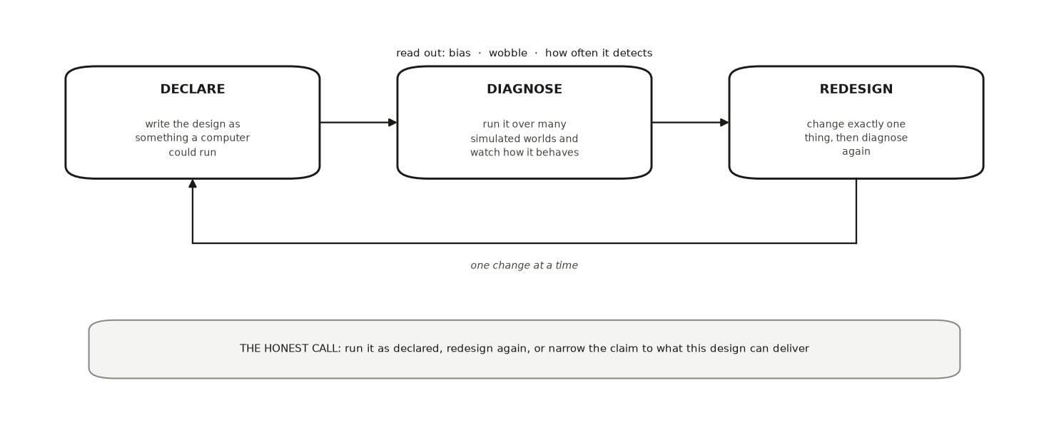
You have already built the four parts of a design. This chapter puts them to the test with a three-step loop this book borrows from RDSS (Research Design in the Social Sciences: Declaration, Diagnosis, and Redesign) (Blair et al. 2023).
Declare means writing your four design parts as something a computer can run: a model that generates fake data, an inquiry it can compute on that fake data, a plan for sampling and assigning conditions, and a rule for turning data into an estimate. Example: code that invents 40 shoppers, flips a coin to give each the new checkout screen, and subtracts the two group averages.
Diagnose means running that declared design many times on fresh simulated worlds and watching how its estimate behaves. Example: run the coin-flip study 2,000 times and collect all 2,000 estimates. Three numbers start the story, and each answers a different worry.
Bias is the average of your errors across the runs, counting direction: each estimate minus the truth, averaged. A design is unbiased when its estimates center on the true answer. Example: the truth is 2, and five runs return 0, 1, 2, 3, and 4. The errors are -2, -1, 0, +1, +2, which average to zero, so bias is zero even though only one run landed on 2. Direction is what makes bias different from plain distance: misses that cancel tell you the design is aimed correctly, while misses that all lean one way tell you it is tilted.
Variance is how much the estimate wobbles from one run to the next. Example: estimates swinging between -5 and +9 around a true value of 2 have high variance. Collecting more of the same kind of data, from the same design, usually shrinks this wobble. It is the one problem size reliably helps.
Power is how often the design detects a real effect, and it means nothing until you say how you would decide (Greenland et al. 2016). A statistical test is the rule you use to decide whether your data conflict enough with “no effect” to call the result real. Example: in the checkout study, a difference-in-means rule: declare an effect when the gap between the two groups is more than about twice its typical run-to-run wobble. The test’s threshold is how demanding that rule is, and it is read across imagined repetitions: at the usual 5 percent setting, a design whose true effect is ZERO would still cry effect in about 5 runs out of 100. The threshold is a property of the rule over many runs, never the chance that your one finding is false. Example: a design that clears that rule in 8 of 100 runs, when the true effect is 2, has 8% power, which is almost useless. Power moves with everything in the declaration: the test, the threshold, the effect you planted, the sample size, and how the world makes noise. Report the whole card beside the number.
Bias, variance, and power are all the same kind of thing: a property of the design read across many simulated runs, never off a single study. Blair, Cooper, Coppock, and Humphreys introduced the term diagnosand for a property of a design you want to diagnose (Blair et al. 2019, 2023). Bias, variance, and power are three of them.
Those three do not exhaust the pile, and fuller diagnoses add more. Two worth knowing by name. Root mean-squared error is the typical size of a miss, with big misses weighted extra. Example: in the five-run example above, the plain average distance is 1.2, but the RMSE is about 1.4, because the two 2-point misses count for more than their share. Coverage is how often the range you report around your estimate actually contains the truth. Example: if you report a range meant to be right 95 times out of 100, coverage checks whether it really is. A design can be unbiased and still miss badly every time, which is exactly why one number is never the whole diagnosis (Morris et al. 2019). The last lesson built these ranges properly; here you only need to know that a diagnosis can ask about them.
Redesign means changing exactly one part in response to the diagnosis, then diagnosing again. Low power from high variance calls for more data. A tilt built into the design, such as who ends up in which group, calls for a different design: more data makes a tilted estimate steadier, not truer.
12.3 A worked example
You work with an online grocery retailer that wants to know whether a one-tap reorder button, which rebuilds a shopper’s last cart in a single press, gets people through checkout faster. Your outcome is seconds-to-complete. Your true effect, in the world you simulate, is that the button shaves 8 seconds off.
You declare it: build shoppers whose baseline checkout times vary a lot, because some browse and some race; flip a coin to assign the button; subtract the two group averages. You diagnose a pilot of 12 shoppers per version. The result is sobering. Bias is near zero, so the design aims true, but the spread is huge because per-person times vary so much, and power comes back under 10%. The design is honest and useless at once. It points at the 8-second gain on average and almost never gets close enough on any single run to prove it.
Now redesign. Variance is the problem, so you raise the sample to 400 per version and diagnose again. Power jumps past 90% and the spread collapses toward the truth. That is variance cured by size. But run one more design as a warning: drop the coin flip and let shoppers opt into the new button themselves. The shoppers who opt in are the frequent, practiced ones who check out faster anyway, so the button gets credit for speed that habit delivered. This confounded design is just as tight at 400 per version, yet it centers on a 14-second gain instead of 8, and no amount of extra data moves it. That gap names the last idea. A randomized design can identify the button’s effect, meaning pin the time gap on the button and rule out other causes, while the confounded one shows only an association, where the two move together but a common cause could explain it.
Diagnosing a design by simulating it many times before running it once is standard practice for evaluating statistical methods (Morris et al. 2019).
The block below declares all three designs and diagnoses each one, which is the whole loop this chapter teaches. Read the bias column and the power column as two different questions.
import numpy as np, pandas as pd
SEED = 464
rng = np.random.default_rng(SEED)

TRUE_EFFECT = -8.0        # seconds the button really saves

def run(n_per_arm, randomize, runs=2000):
    """Declare a design once, then diagnose it by running it many times."""
    out = []
    for _ in range(runs):
        base = rng.normal(150, 32, size=2 * n_per_arm)     # people differ a lot
        if randomize:
            treated = rng.random(2 * n_per_arm) < 0.5
        else:                       # shoppers opt in — the fast ones do
            treated = rng.random(2 * n_per_arm) < 1 / (
                1 + np.exp((base - 150) / 170))
        secs = base + TRUE_EFFECT * treated + rng.normal(0, 8, size=2 * n_per_arm)
        out.append(secs[treated].mean() - secs[~treated].mean())
    est = np.array(out)
    se = est.std(ddof=1)
    return {"estimate": est.mean(), "bias": est.mean() - TRUE_EFFECT,
            "power": float((np.abs(est) > 1.96 * se).mean())}

designs = {"pilot, randomized, 12/arm": run(12, True),
           "randomized, 400/arm": run(400, True),
           "opt-in, 400/arm": run(400, False)}
print(pd.DataFrame(designs).T.round(2).to_string())
print("\nsize cured the variance. it did nothing for the opt-in design's bias")
12.4 Preregistration and the pre-analysis plan
Your checkout design passed its diagnosis at 400 shoppers per version. Before the first shopper taps anything, you do one more thing with it: you post it where anyone can read it, with a date stamp you cannot edit later.
Preregistration is a public, time-stamped record of your question and your plan, filed before you see the outcomes (Nosek et al. 2018). Example: a dated entry on a public registry saying that you will compare checkout seconds between shoppers randomly shown the reorder button and shoppers who were not.
A pre-analysis plan is the detailed part of that record: every choice that turns raw data into your reported number, written precise enough that a stranger could compute it. Example: “The outcome is seconds from cart to payment for completed checkouts. The estimate is the difference in group means. We flag an effect when that gap exceeds 1.96 standard errors. Phones versus laptops is the only subgroup we will test.” RDSS recommends that the plan center on the design declaration itself, the same model, inquiry, data strategy, and answer strategy you just wrote as code, ideally with mock analyses run on simulated data (Blair et al. 2023). Humphreys, Sanchez de la Sierra, and van der Windt went a step further: they wrote a complete mock report of their field experiment, running every planned analysis on fake treatment assignments before the real analysis (Humphreys et al. 2013). Your declaration from this chapter is most of a plan already.
Why bother, if you intend to be honest? Because the choices you leave open keep multiplying after the data arrive, and each one looks reasonable in the moment. Humphreys and his coauthors showed that fixing only the outcome and the treatment in advance still leaves wide room to go fishing through covariates and subgroups (Humphreys et al. 2013). The block below runs the checkout study in a world where the button does nothing at all. One analyst reports the full-sample comparison she wrote down in advance. Another looks at the data and then reports whichever of five sensible cuts clears the bar: everyone, phone shoppers, laptop shoppers, returning shoppers, or everyone after dropping checkouts slower than 200 seconds.
import numpy as np
SEED = 464
rng = np.random.default_rng(SEED)

# The button does NOTHING here: the true effect is ZERO seconds.
n, runs = 400, 4_000            # about 400 shoppers per version, 4,000 runs

def flags(secs, treated, keep):
    """Difference in means, flagged when it exceeds 1.96 standard errors."""
    a, b = secs[keep & treated], secs[keep & ~treated]
    se = np.sqrt(a.var(ddof=1) / len(a) + b.var(ddof=1) / len(b))
    return abs(a.mean() - b.mean()) > 1.96 * se

planned = forked = 0
for _ in range(runs):
    secs = rng.normal(150, 32, size=2 * n)
    phone = rng.random(2 * n) < 0.5
    returning = rng.random(2 * n) < 0.5
    treated = rng.random(2 * n) < 0.5
    everyone = np.full(2 * n, True)
    paths = [everyone, phone, ~phone, returning, secs < 200]  # the last one drops
    hits = [flags(secs, treated, keep) for keep in paths]     # slow checkouts
    planned += hits[0]          # the one analysis written down in advance
    forked += any(hits)         # report whichever path "worked"
print(f"false alarms, planned analysis : {planned / runs:.1%}")
print(f"false alarms, best of 5 paths  : {forked / runs:.1%}")
print("\nfive sensible choices, made after looking, loosen a 5% rule")
The planned analysis cries effect in 4.5% of the 4,000 runs, close to the 5 percent its threshold promises. The analyst who picks a path after looking cries effect in 16.9%, almost four times as often, for a button that saves no time. With 4,000 runs, each rate has a simulation standard error below one percentage point, so the gap is no accident of this seed. How wide it grows in your study depends on how many paths you leave open. Nothing in the second analyst’s report shows the forks she walked past.
A plan can change, as long as the change is on the record. A deviation is any place where what you did differs from what you planned. Example: the retailer’s app update changes how checkout time is logged halfway through, so you switch to the server’s timestamp. Deviations are common, and the fix is to report each one: what changed, why, and whether you had seen outcomes when you decided (Nosek et al. 2018). Readers can then judge the change for themselves. A silent change is the problem.
The plan also sorts your findings into two honest piles. A confirmatory analysis is one you committed to in the plan; an exploratory analysis is one you chose after seeing data. Example: the phone-versus-laptop split is confirmatory; a pattern you notice by day of week is exploratory. Both belong in your report. What differs is what the threshold can tell a reader. For a committed test, the reader knows how many chances you gave yourself, so the stated 5 percent means something, provided the test’s own assumptions hold. For an exploratory result, nobody knows how many paths were tried, so the same threshold no longer says how often such a finding turns up by chance (Nosek et al. 2018). The committed rate also holds one test at a time. The example plan above makes two tests, the full sample and the phone-versus-laptop split, so it should also say how it handles that second chance, for instance with a stricter threshold. Label every result with the pile it came from.
When the data already exist, as with a public election file in political science or a firm’s past sales records, a time stamp cannot show you never peeked. Then you say plainly what you have and have not looked at, write the plan before opening the outcome columns, or split the file and seal one part until your exploring is done (Nosek et al. 2018). Your credibility rests on that record, and a reader may still discount it.
Some journals go further with registered reports, a format in which reviewers judge your question and plan before the results exist and the journal can accept the paper in principle, whatever the results turn out to be, provided you carry out the approved plan (Chambers 2013). Neither format makes a design sound. The opt-in checkout design, preregistered word for word, still centers on 14 seconds. And a vague plan leaves the forks open: when Ofosu and Posner read 195 plans filed on two social-science registries in 2011–2016, they found wide variation in whether the plans were clear and precise enough to stop fishing (Ofosu and Posner 2023).
An AI tool is a fast drafter here. Give it your declared code and it will produce a plan template and list the choices your declaration left unstated, such as exclusions, missing outcomes, and subgroups. It also fails in two predictable ways. It fills gaps silently with its own defaults, and it writes soft sentences like “we will explore heterogeneity” that commit you to nothing. After the data arrive, an agentic tool can run dozens of specifications in seconds, which makes the forking paths cheaper than ever. Which analysis is primary, and the decision to post the plan with your name on it, stay with you. Systematic reviews register their protocols in the same spirit; the evidence-synthesis route shows what that plan contains.
12.5 An AI failure case
You paste your confounded observational design and ask, “My estimate is noisy. What should I do?” The tool answers with confidence: “Collect more observations to tighten your estimate.” That sounds obviously right and is exactly wrong for your case. Your problem is bias from self-selection, not variance, and more data only makes a biased estimate a more precise wrong number. You catch it the way this chapter teaches: run the confounded design in simulation at a large sample and watch the estimates cluster tightly around 14 seconds when the truth is 8. The spread shrank; the error did not. That is the plausible-but-wrong-method failure, and your own diagnosis unmasks it.
12.6 It is your turn
You are working inside Studio 4: Declare and diagnose provisionally. Keep what you write here; the studio’s milestone chapter is where it joins the other lessons’ pieces into one artifact you can defend.
You have four design parts on paper. This step asks whether they would survive contact with the world, while a bad answer is still free. The declare-and-diagnose loop, and the word “diagnosand” for the properties you read out of it, come from Blair, Cooper, Coppock, and Humphreys, developed at book length in RDSS.
The hands-on half of this section lives in the chapter’s companion notebook: open it in Colab with the badge at the top, and work the steps there.
Commit your own expectation first, then delegate. Each prompt below leaves you a draft you still have to check. Simulation is where the loop gets fastest and most dangerous at once: modern coding assistants will write the script, run it, read the error, and patch it without waiting for you, and they will happily converge on code that runs cleanly while declaring a different design than yours. Let the tool own the typing. Keep ownership of the true effect you plant and the numbers you read out.
Three calls stay yours. Which world your question assumes, the model you declare, is a claim about reality no tool can make for you. Which single quantity you name as your inquiry decides what “success” even means. And the honest call of whether to run a design your own diagnosis says is too weak is a judgment you sign your name to. An AI can propose threats and draft simulation code, but it cannot decide that your under-powered study is worth months of your life anyway.
Declare your design as something that can be run. If you can code it, write the smallest script that builds a world where you set the true effect, draws your sample, applies your answer strategy, and prints one estimate. If you cannot code it yet, declare it in words precise enough that someone else could: state the true effect you are assuming, the number of units, and the exact arithmetic.
When you are ready to delegate this step:
Act as a simulation assistant. Here is my declared design in words:
[model, inquiry, data strategy, answer strategy]. Write the smallest Python
that builds a world where I set the true effect, runs the design many times,
and reports bias, variance, and power. List every assumption your code makes
about my design that I did not state.
After running, verify (counters plausible-but-wrong-method): re-run it with the true effect set to zero and confirm it “detects” an effect only about as often as your significance threshold allows. A simulation that fires on a zero effect is declaring a different design than yours.
Diagnose it. Run it a few thousand times and read three numbers: bias (do the estimates center on the truth you planted?), variance (how wide is the spread?), and power (how often does it clear your stated threshold?). Write down the test and threshold you used, or the power number means nothing. If you cannot simulate yet, record each number as “not estimated” and reason in words about direction instead: which way you expect the tilt, and what would widen the spread. Label that reasoning as reasoning. A number you did not compute is not a diagnosis.
Name the worst of the three, and say which kind of problem it is. Wobble and low power often yield to a bigger sample, though not only to it: sharper measurement, better-balanced groups, and a stronger treatment contrast all buy power too. A tilt in who ends up where is a design problem, and a bigger sample makes it more precise rather than less wrong.
When you are ready to delegate this step:
Here is my diagnosed design and its numbers: [bias, variance, power]. List the
threats to any conclusion from one run as a table: threat, whether it is a
bias / variance / power problem, and the single redesign that reduces it most.
After running, verify (counters illusion of completeness): check the table against your own printed diagnosis. The killer your numbers already proved must be the top row; a tidy six-threat list that never names it missed the point.
Redesign once. Change exactly one thing, the one your diagnosis points at, and diagnose again. Record both diagnoses side by side so the improvement is visible.
Make the honest call in one sentence: run it as redesigned, redesign again, or narrow the claim to what this design can actually deliver. All three are respectable outcomes. Pretending you never checked is not.
When you are ready to delegate this step:
Argue against my claim that this design is strong enough to run. As a hostile
methodologist, name the one diagnosand I am most likely fooling myself about,
and the observation that would expose it.
After running, verify (counters sycophantic agreement): if it praises the design without a single objection, discard the answer and diagnose again yourself.
Log both diagnoses in your AI Research Ledger, and verify the key number with a named method from the Verification Guide; simulation is the method for a claim about how a procedure behaves, and a causal diagram is the second check if your inquiry uses the word causes. An AI reviewer may run the diagnosis with you; the decision to run, fix, or narrow stays yours.