MGMT 47400: Predictive Analytics
Tree Based Methods
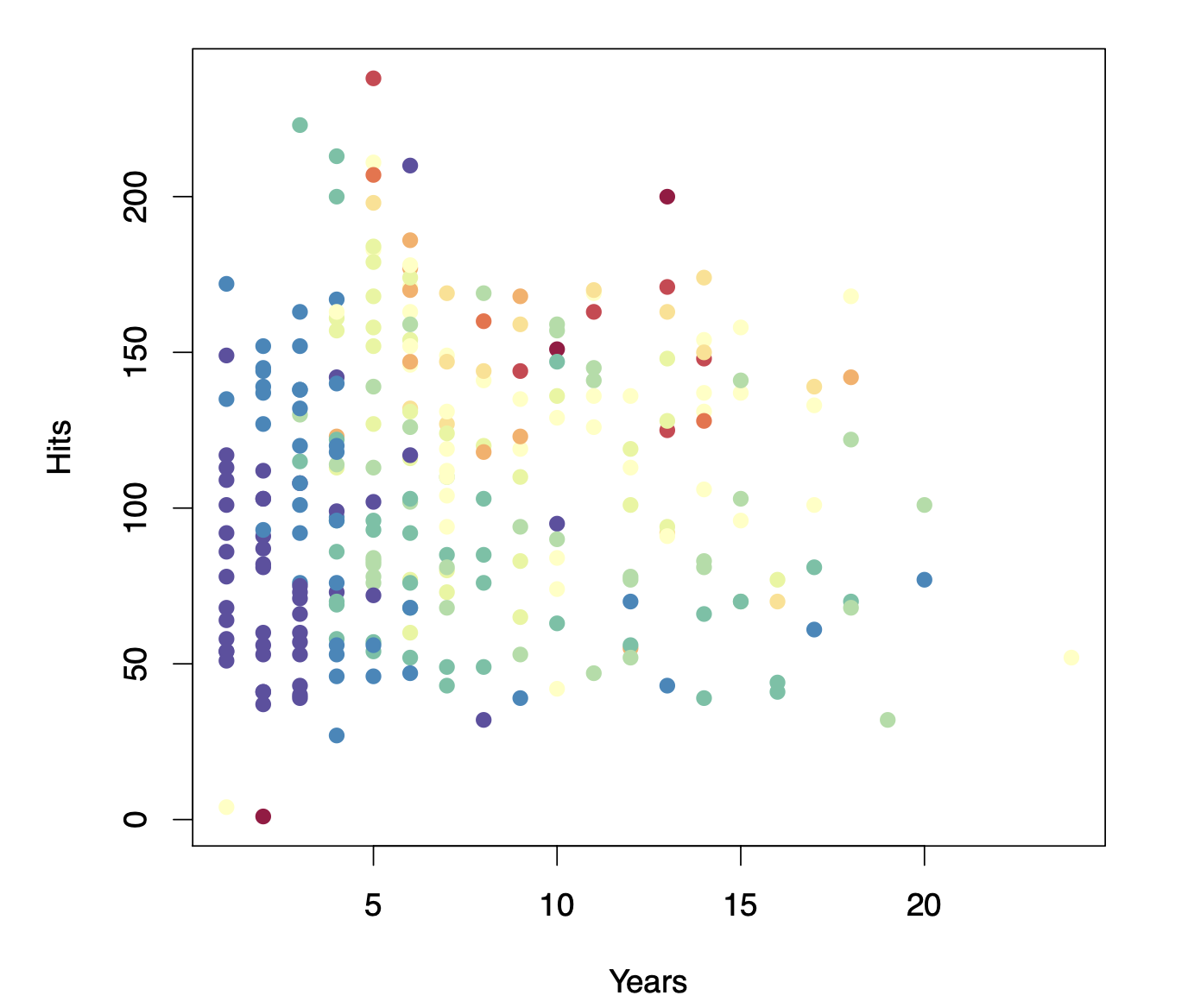
Decision tree for these data

The top node represents the full dataset.
The first split is based on years of experience:
- Players with less than 4.5 years → Left branch.
- Players with more than 4.5 years → Right branch.
This split closely aligns with our initial estimate of 5 years.
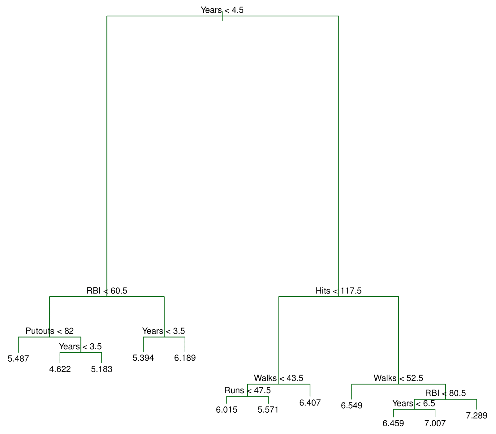
Among players with more than 4.5 years, the tree applies a second split:
- Fewer than 117.5 hits → Left branch.
- More than 117.5 hits → Right branch.
This recursive splitting refines the salary prediction.
What Do the Numbers Represent?
The values at the bottom nodes indicate the average log salary of players in that group.
Since a log transformation was applied, these values represent average log salaries rather than raw salaries.
Final Segmentation
The decision tree ultimately divides players into three distinct salary groups:
- Highest salary
- Medium salary
- Lowest salary
These categories closely match—though not exactly—the three regions we initially identified.
By systematically applying these splits, decision trees segment data into meaningful, homogeneous groups.
The final tree has two internal nodes and three terminal nodes (leaves). The number in each leaf is the mean of the response for the observations that fall there.
Results
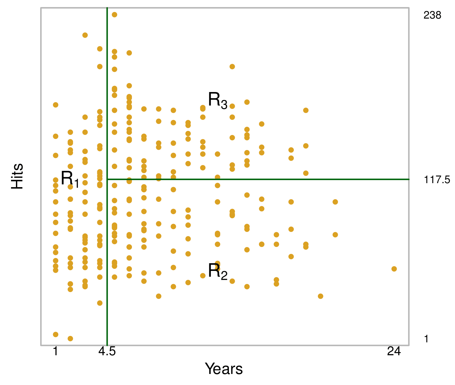
The tree stratifies or segments the players into three regions of predictor space:
\[ R_1 = \{X \ | \ \text{Years} < 4.5\} \]
\[ R_2 = \{X \ | \ \text{Years} \geq 4.5, \text{Hits} < 117.5\} \]
\[ R_3 = \{X \ | \ \text{Years} \geq 4.5, \text{Hits} \geq 117.5\} \]
Details— Continued
We first select the predictor \(X_j\) and the cutpoint \(s\) such that splitting the predictor space into the regions \(\{X | X_j < s\}\) and \(\{X | X_j \geq s\}\) leads to the greatest possible reduction in RSS.
Next, we repeat the process, looking for the best predictor and best cutpoint in order to split the data further so as to minimize the RSS within each of the resulting regions.
However, this time, instead of splitting the entire predictor space, we split one of the two previously identified regions. We now have three regions.
Again, we look to split one of these three regions further, so as to minimize the RSS. The process continues until a stopping criterion is reached; for instance, we may continue until no region contains more than five observations.
Predictions: Example
A five-region example
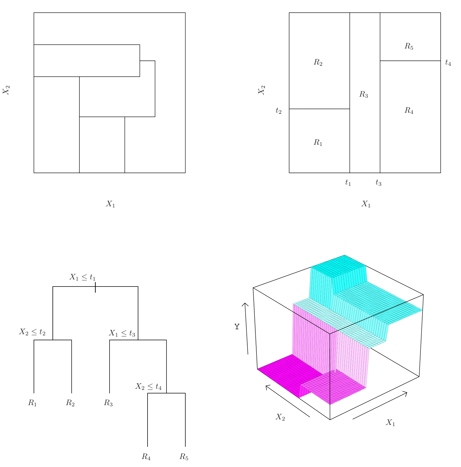
Top Left: A partition of two-dimensional feature space that could not result from recursive binary splitting.
Top Right: The output of recursive binary splitting on a two-dimensional example.
Bottom Left: A tree corresponding to the partition in the top right panel.
Bottom Right: A perspective plot of the prediction surface corresponding to that tree.
Baseball example: The Full Tree Before Pruning
Baseball example: Cross Validation for the Prune Tree
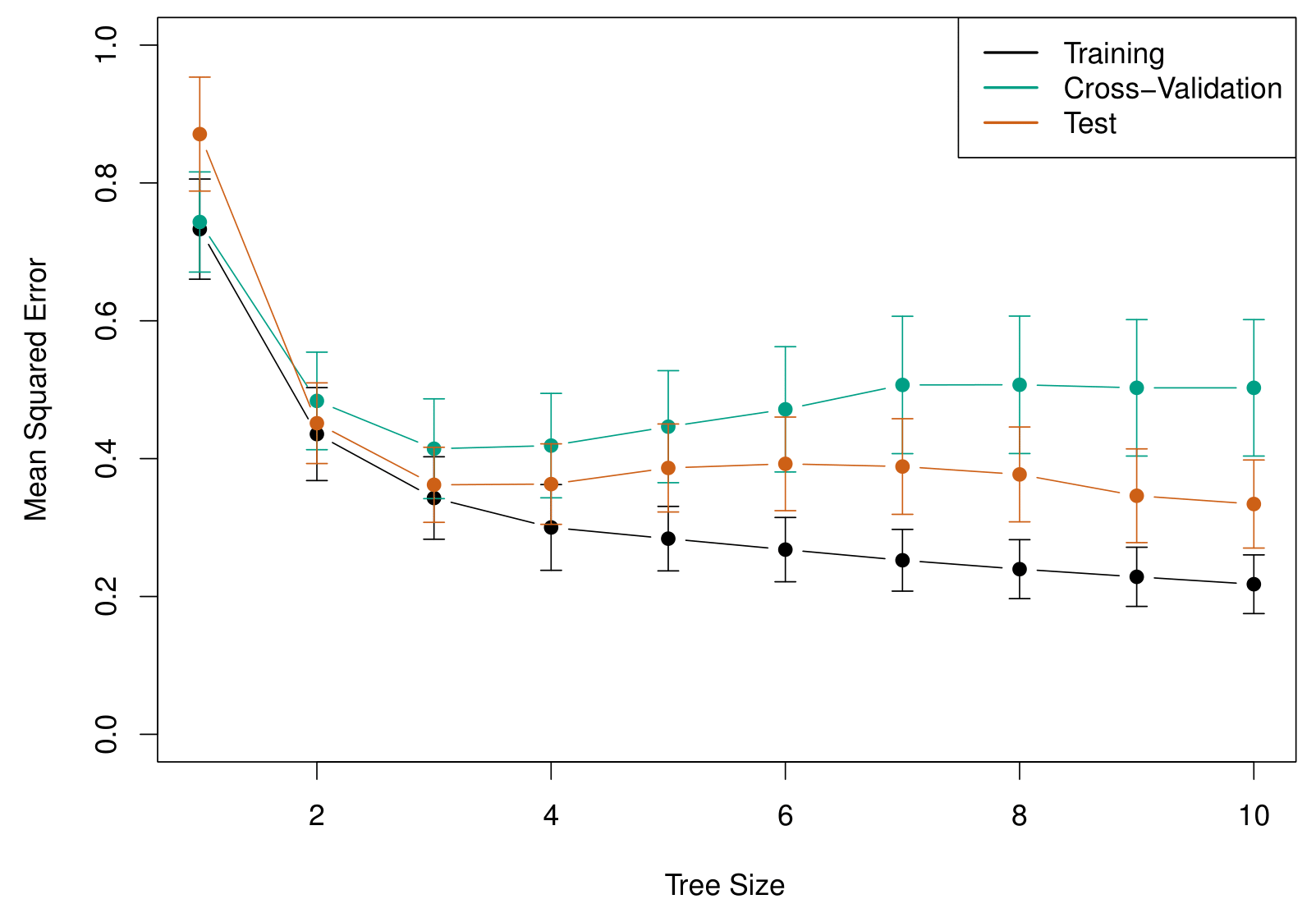
Along the horizontal axis, we have tree size, which is controlled by the alpha parameter (\(\alpha\)). This parameter directly influences the complexity of the decision tree.
When \(\alpha = 0\), there is no penalty on tree size, meaning the model grows to its largest possible tree, which in this case contains 12 terminal nodes.
As \(\alpha\) increases, a stronger penalty is applied to larger trees, gradually reducing the number of terminal nodes.
As \(\alpha\) continues to increase, the model prunes away more splits, simplifying the tree structure.
At the extreme, when \(\alpha\) is large enough, the tree is reduced to a single node, meaning no splits occur, and the model collapses into a single global mean prediction.
The green curve is what we get from cross validation and it’s minimized at around three terminal nodes!
Example: Heart data
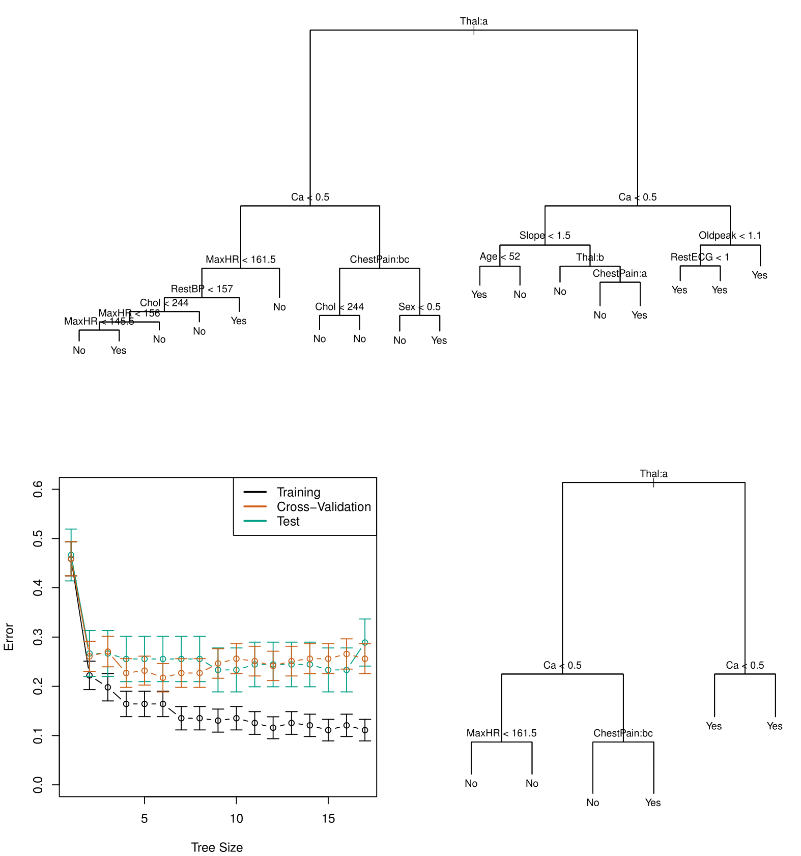
At the top, we see the fully grown tree.
- The first split occurs on FEL (a thallium stress test), followed by splits on CA (calcium). The terminal nodes classify observations as “No” (no heart disease) or “Yes” (heart disease) based on majority class.
- Some terminal nodes with the same classification still have splits. This suggests that while both nodes predict “No,” one is purer than the other, as identified by the Gini index.
Since this tree is likely too complex, cross-validation was used to find an optimal size.
- The right panel shows training, validation, and test errors, with the cross-validation error curve guiding the selection of a tree size. A tree with six terminal nodes performed best, balancing complexity and accuracy.
The pruned tree (size six) is shown on the right, derived using the cost-complexity parameter (\(\alpha\)). This subtree of the original tree achieved an estimated 25% classification error—a significant improvement in generalization.
Trees Versus Linear Models
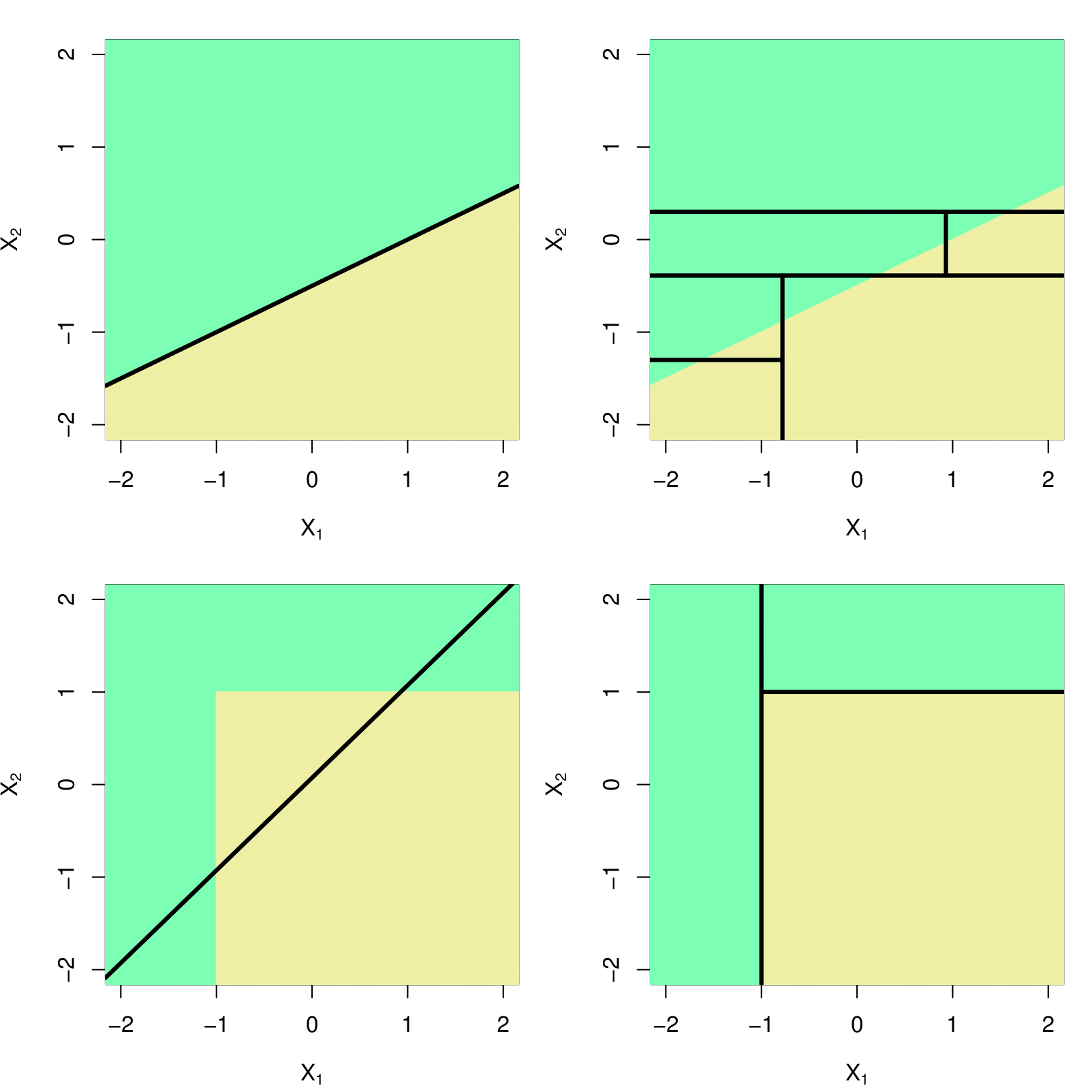
- Top Row: True linear boundary;
- Bottom row: true non-linear boundary.
- Left column: Linear model;
- Right column: Tree-based model.
Bagging the Heart data
Bagging and Random Forest results.
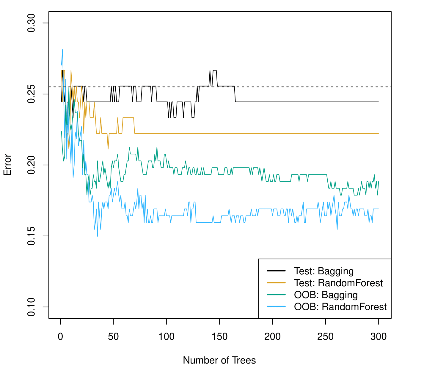
The dashed line indicates the test error resulting from a single classification tree.
The test error (black and orange) is shown as a function of \(B\), the number of bootstrapped training sets used.
Random forests were applied with \(m = \sqrt{p}\).
The green and blue traces show the Out-of-Bag (OOB) error, which in this case is considerably lower.
Results: Gene Expression Data
Results from random forests for the fifteen-class gene expression data set with \(p = 500\) predictors.
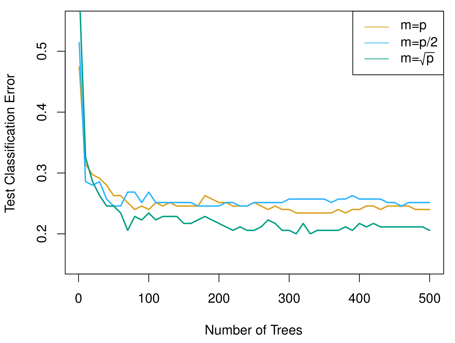
The test error is displayed as a function of the number of trees. Each colored line corresponds to a different value of \(m\), the number of predictors available for splitting at each interior tree node.
Random forests (\(m < p\)) lead to a slight improvement over bagging (\(m = p\)). A single classification tree has an error rate of 45.7%.
Example: Gene expression data continued
Results from performing boosting and random forests on the fifteen-class gene expression data set in order to predict cancer versus normal.
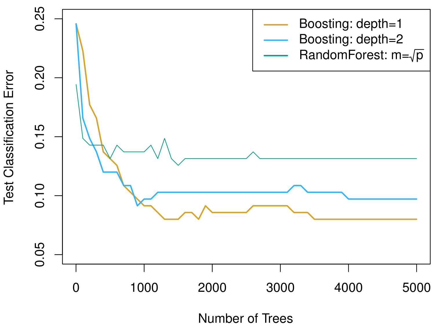
The test error is displayed as a function of the number of trees.
For the two boosted models, \(\lambda = 0.01\). Depth-1 trees, when a single split where applied, slightly outperform depth-2 trees, and both outperform the random forest, although the standard errors are around 0.02, making none of these differences significant.
The test error rate for a single tree is 24%.
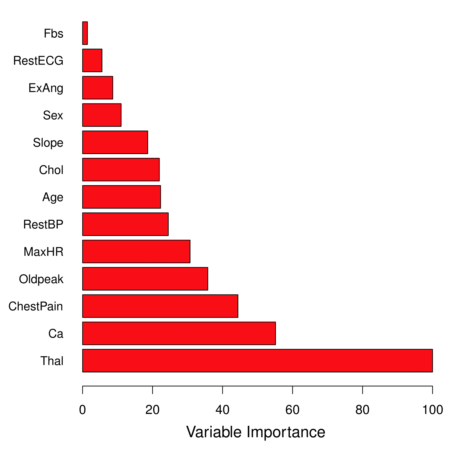
Variable Importance Measure
For bagged/RF regression trees:
Record the total amount that the RSS is decreased due to splits over a given predictor, averaged over all \(B\) trees.
A large value indicates an important predictor.
For bagged/RF classification trees:
- Add up the total amount that the Gini index is decreased by splits over a given predictor, averaged over all \(B\) trees.
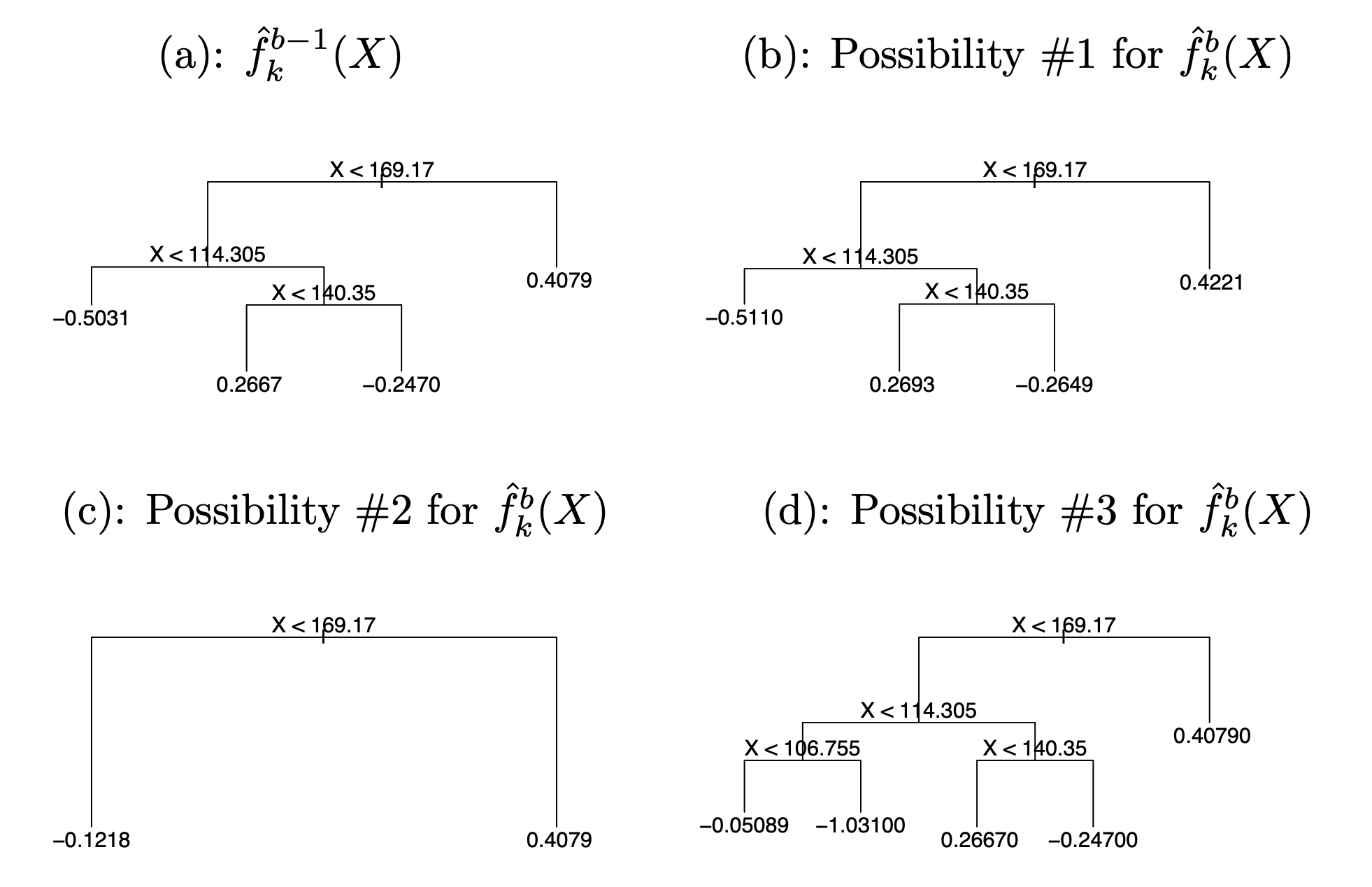
BART Algorithm Intuition
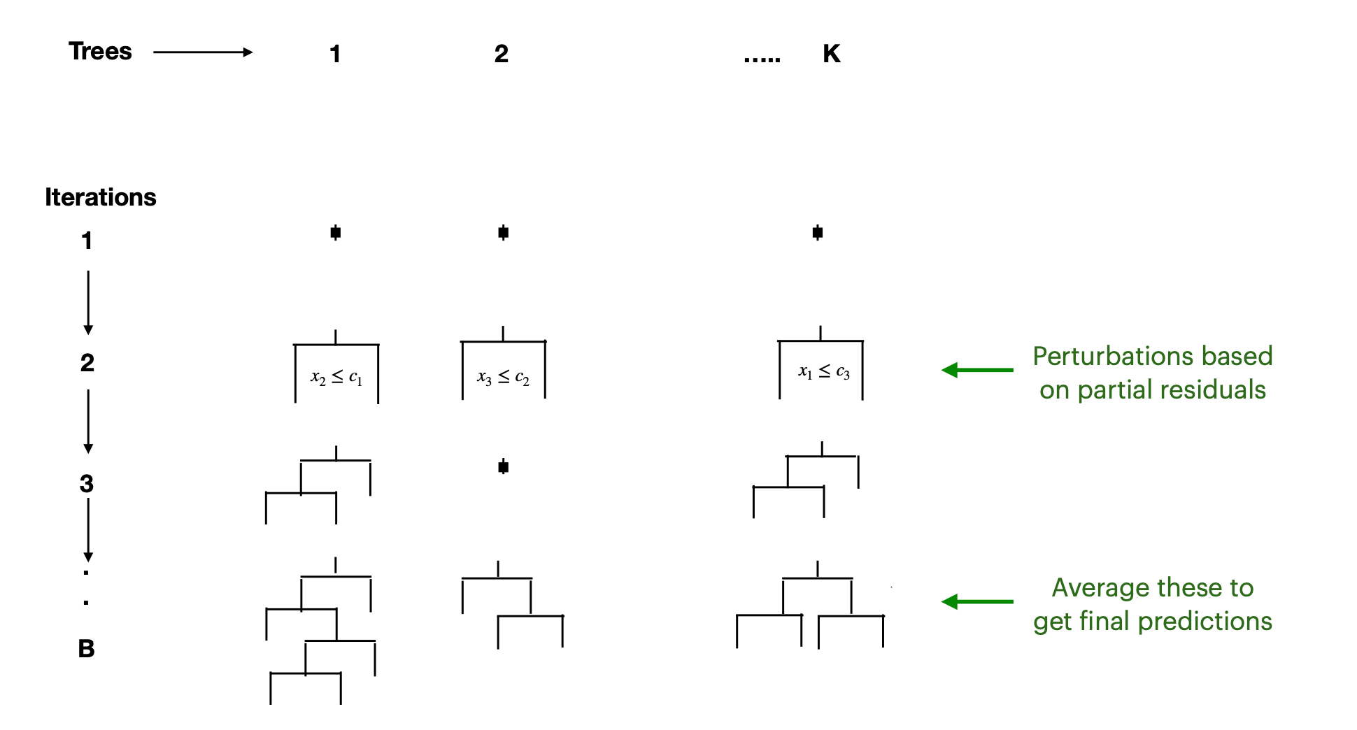
Examples of possible perturbations to a tree
BART applied to the Heart data

\(K = 200\) trees; the number of iterations is increased to 10,000.
During the initial iterations (in gray), the test and training errors jump around a bit.
After this initial burn-in period, the error rates settle down.
The tree perturbation process largely avoids overfitting.