What is a classification problem?

Classification involves categorizing data into predefined classes or groups based on their features.
Classification
Qualitative variables take values in an unordered set \(C\), such as:
- \(\text{eye color} \in \{\text{brown}, \text{blue}, \text{green}\}\)
- \(\text{email} \in \{\text{spam}, \text{ham}\}\)
Given a feature vector \(X\) and a qualitative response \(Y\) taking values in the set \(C\), the classification task is to build a function \(C(X)\) that takes as input the feature vector \(X\) and predicts its value for \(Y\); i.e. \(C(X) \in C\).
Often, we are more interested in estimating the probabilities that \(X\) belongs to each category in \(C\).
- For example, it is more valuable to have an estimate of the probability that an insurance claim is fraudulent, than a classification as fraudulent or not.
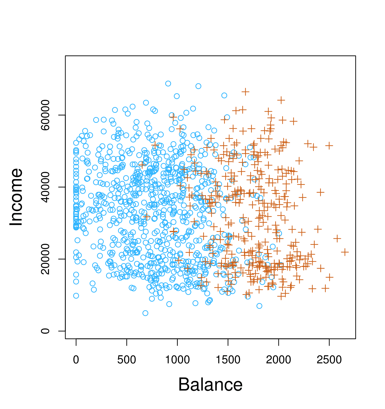
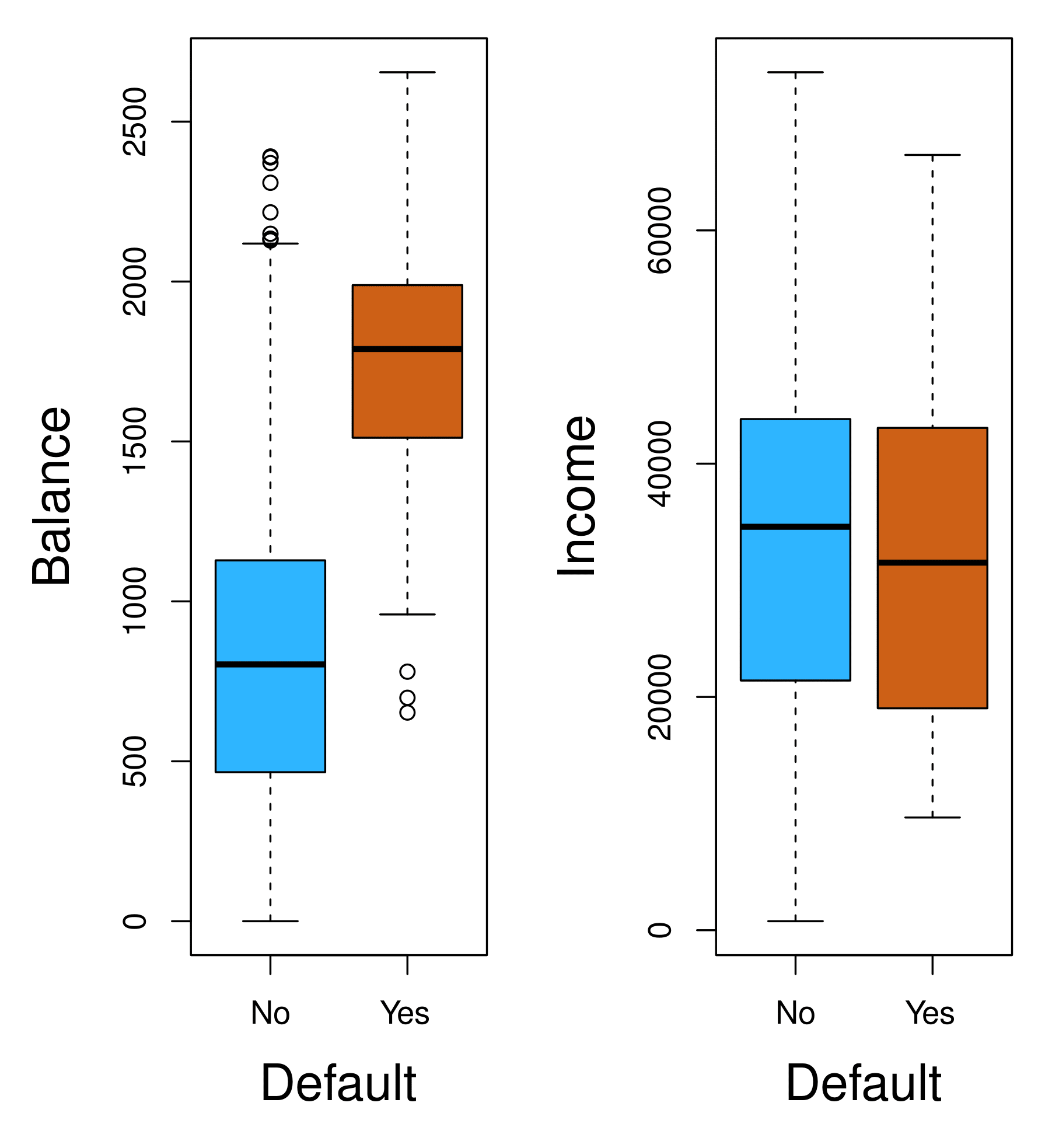
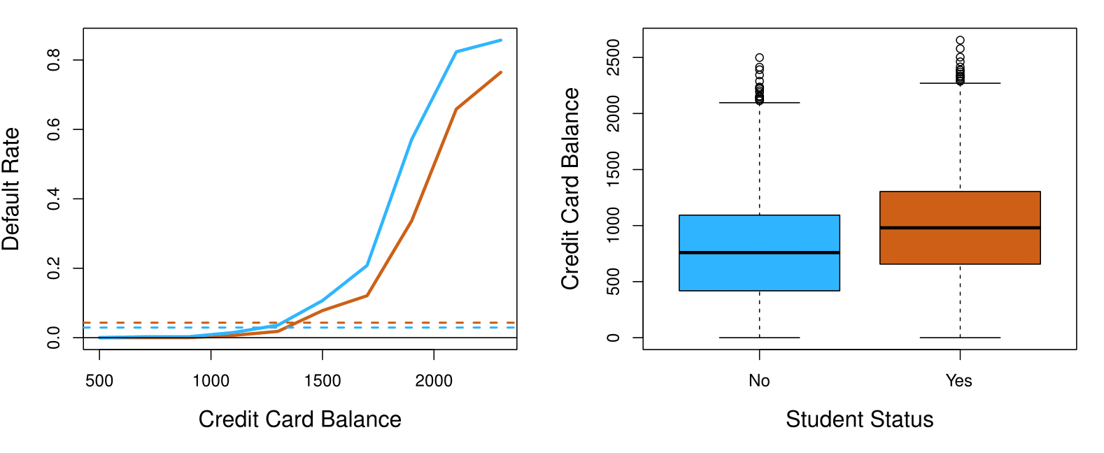
Example: Credit Card Default
Scatter plot of income vs. balance with markers indicating whether a person defaulted (e.g., “+” for defaulted, “o” for not defaulted).
Boxplots comparing balance and income for default (“Yes”) vs. no default (“No”).
Can we use Linear Regression?
Suppose for the Default classification task that we code:
\[
Y =
\begin{cases}
0 & \text{if No} \\
1 & \text{if Yes.}
\end{cases}
\]
Can we simply perform a linear regression of \(Y\) on \(X\) and classify as Yes if \(\hat{Y} > 0.5\)?
- In this case of a binary outcome, linear regression does a good job as a classifier and is equivalent to linear discriminant analysis, which we discuss later.
- Since in the population \(E(Y|X = x) = \Pr(Y = 1|X = x)\), we might think that regression is perfect for this task.
- However, linear regression might produce probabilities less than zero or greater than one. Logistic regression is more appropriate.
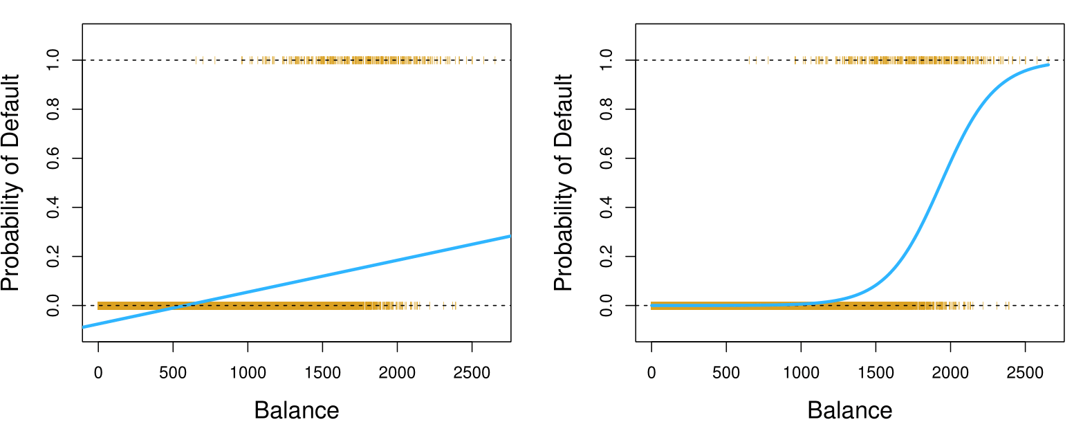
Linear versus Logistic Regression: Probability of Default
The orange marks indicate the response \(Y\), either 0 or 1.
Linear regression does not estimate \(\Pr(Y = 1|X)\) well.
Logistic regression seems well-suited to the task.
Linear Regression continued
Now suppose we have a response variable with three possible values. A patient presents at the emergency room, and we must classify them according to their symptoms.
\[
Y =
\begin{cases}
1 & \text{if stroke;} \\
2 & \text{if drug overdose;} \\
3 & \text{if epileptic seizure.}
\end{cases}
\]
This coding suggests an ordering, and in fact implies that the difference between stroke and drug overdose is the same as between drug overdose and epileptic seizure.
Linear regression is not appropriate here. Multiclass Logistic Regression or Discriminant Analysis are more appropriate.
Logistic Regression
Let’s write \(p(X) = \Pr(Y = 1|X)\) for short and consider using balance to predict default. Logistic regression uses the form:
\[
p(X) = \frac{e^{\beta_0 + \beta_1 X}}{1 + e^{\beta_0 + \beta_1 X}}.
\]
\((e \approx 2.71828)\) is a mathematical constant Euler’s number.
It is easy to see that no matter what values \(\beta_0\), \(\beta_1\), or \(X\) take, \(p(X)\) will have values between 0 and 1.
A bit of rearrangement gives:
\[
\log\left(\frac{p(X)}{1 - p(X)}\right) = \beta_0 + \beta_1 X.
\]
This monotone transformation is called the log odds or logit transformation of \(p(X)\). (By log, we mean natural log: \(\ln\).)
Linear versus Logistic Regression
Linear versus Logistic Regression
Logistic regression ensures that our estimate for \(p(X)\) lies between 0 and 1.
Maximum Likelihood
We use maximum likelihood to estimate the parameters.
\[
\ell(\beta_0, \beta) = \prod_{i:y_i=1} p(x_i) \prod_{i:y_i=0} (1 - p(x_i)).
\]
- The Maximum Likelihood Estimation (MLE) is a method used to estimate the parameters of a model by maximizing the likelihood function, which measures how likely the observed data is given the parameters.
The likelihood function is based on the probability distribution of the data. If you assume that the data points are independent, the likelihood function is the product of the probabilities of each observation.
Considering a data series of observed zeros and ones, and a model for the probabilities involving parameters (e.g., \(\beta_0\) and \(\beta_1\)), for any specific parameter values, we can compute the probability of observing the data.
Since the observations are assumed to be independent, the joint probability of the observed sequence is the product of the probabilities for each observation. For each “1,” we use the model’s predicted probability, \(p(x_i)\), and for each “0,” we use \(1 - p(x_i)\).
The goal of MLE is to find the parameter values that maximize this joint probability, as they make the observed data most likely to have occurred.
Maximum Likelihood Estimation (MLE) Example: Coin Flipping
Suppose you are flipping a coin, and you observe 5 heads out of 10 flips. The coin’s bias (the probability of heads) is \(p\), and you want to estimate \(p\).
The probability of observing a single outcome (heads or tails) follows the Bernoulli distribution:
\[
P(\text{Heads or Tails}) = p^x (1-p)^{1-x}, \quad \text{where } x = 1 \text{ for heads, } x = 0 \text{ for tails.}
\]
For 10 independent flips, the likelihood function is:
\[
L(p) = P(\text{data} \mid p) = \prod_{i=1}^{10} p^{x_i}(1-p)^{1-x_i}.
\]
If there are 5 heads (\(x=1\)) and 5 tails (\(x=0\)):
\[
L(p) = p^5 (1-p)^5.
\]
Maximum Likelihood Estimation (MLE) Example: Coin Flipping
Simplify with the Log-Likelihood
Since multiplying probabilities can result in very small numbers, we take the logarithm of the likelihood (log-likelihood). The logarithm simplifies the product into a sum:
\[
\ell(p) = \log L(p) = \log \left(p^5 (1-p)^5\right) = 5\log(p) + 5\log(1-p).
\]
Maximum Likelihood Estimation (MLE) Example: Coin Flipping
Maximize the Log-Likelihood
To find the value of \(p\) that maximizes \(\ell(p)\), take the derivative of the log-likelihood with respect to \(p\) and set it to zero:
\[
\frac{\partial\ell(p)}{\partial p} = \frac{5}{p} - \frac{5}{1-p} = 0.
\]
Simplify:
\[
\frac{5}{p} = \frac{5}{1-p}.
\]
Solve for \(p\):
\[
1 - p = p \quad \Rightarrow \quad 1 = 2p \quad \Rightarrow \quad p = 0.5.
\]
Maximum Likelihood Estimation (MLE) Example: Coin Flipping
To confirm that \(p = 0.5\) is the maximum, you can check the second derivative of the log-likelihood (concavity) or use numerical methods.
In our example, \(p = 0.5\) makes sense intuitively because the data (5 heads out of 10 flips) suggests the coin is unbiased.
The maximum likelihood estimate of \(p\) is \(0.5\). The MLE method finds the parameter values that make the observed data most likely, given the assumed probability model.
Maximum Likelihood Estimation (MLE) Example: Estimating the Mean of a Normal Distribution
Assumptions:
- Data \(x_1, x_2, \dots, x_n\) are drawn from a normal distribution with:
\[
f(x | \mu, \sigma) = \frac{1}{\sqrt{2\pi \sigma^2}} e^{-\frac{(x - \mu)^2}{2\sigma^2}}
\]
- Assume \(\sigma\) is known (say, \(\sigma = 1\)) and we want to estimate \(\mu\).
Maximum Likelihood Estimation (MLE) Example: Estimating the Mean of a Normal Distribution
The likelihood for \(n\) independent observations is:
\[
L(\mu) = \prod_{i=1}^n \frac{1}{\sqrt{2\pi}} e^{-\frac{(x_i - \mu)^2}{2}}
\]
Taking the natural log:
\[
\ell(\mu) = \log L(\mu) = \sum_{i=1}^n \left[ -\frac{1}{2} \log(2\pi) - \frac{(x_i - \mu)^2}{2} \right]
\]
Simplify (since \(-\frac{1}{2} \log(2\pi)\) is constant):
\[
\ell(\mu) = -\frac{n}{2} \log(2\pi) - \frac{1}{2} \sum_{i=1}^n (x_i - \mu)^2
\]
Maximum Likelihood Estimation (MLE) Example: Estimating the Mean of a Normal Distribution
Differentiate with respect to \(\mu\):
\[
\frac{\partial \ell(\mu)}{\partial \mu} = -\sum_{i=1}^n (x_i - \mu)
\] Set this to zero:
\[
\sum_{i=1}^n (x_i - \mu) = 0
\]
Solve for \(\mu\):
\[
\mu = \frac{1}{n} \sum_{i=1}^n x_i
\]
The MLE for the mean \(\mu\) is simply the sample mean:
\[
\hat{\mu} = \frac{1}{n} \sum_{i=1}^n x_i
\]
Discriminant Analysis
Here the approach is to model the distribution of \(X\) in each of the classes separately, and then use Bayes theorem to flip things around and obtain \(\Pr(Y \mid X)\).
When we use normal (Gaussian) distributions for each class, this leads to linear or quadratic discriminant analysis.
However, this approach is quite general, and other distributions can be used as well. We will focus on normal distributions as input for \(f_k(x)\).
Bayes Theorem for Classification
Thomas Bayes was a famous mathematician whose name represents a big subfield of statistical and probabilistic modeling. Here we focus on a simple result, known as Bayes theorem:
\[
\Pr(Y = k \mid X = x) = \frac{\Pr(X = x \mid Y = k) \cdot \Pr(Y = k)}{\Pr(X = x)}
\]
One writes this slightly differently for discriminant analysis:
\[
\Pr(Y = k \mid X = x) = \frac{\pi_k f_k(x)}{\sum_{\ell=1}^K \pi_\ell f_\ell(x)}, \quad \text{where}
\]
\(f_k(x) = \Pr(X = x \mid Y = k)\) is the density for \(X\) in class \(k\). Here we will use normal densities for these, separately in each class.
\(\pi_k = \Pr(Y = k)\) is the marginal or prior probability for class \(k\).
Bayes’ Theorem: Explanation
It describes the probability of an event, based on prior knowledge of conditions that might be related to the event.
\[
P(A|B) = \frac{P(B|A) \cdot P(A)}{P(B)}
\]
\(P(A|B)\): Posterior probability - Probability of event \(A\) occurring given that \(B\) is true — updated probability after the evidence is considered.
\(P(A)\): Prior probability - Initial probability of event \(A\) — the probability before the evidence is considered.
\(P(B|A)\): Likelihood - Probability of observing event \(B\) given that \(A\) is true.
\(P(B)\): Marginal probability - Total probability of the evidence, event \(B\).
Understanding Conditional Probability
Conditional probability is the probability of an event occurring given that another event has already occurred.
Definition:
\[
P(A|B) = \frac{P(A \cap B)}{P(B)}
\]
is the probability of event \(A\) occurring given that \(B\) is true.
- Interpretation: How likely is \(A\) if we know that \(B\) happens?
What is Joint Probability?
Joint probability refers to the probability of two events occurring together.
Definition: \(P(A \cap B)\) is the probability that both \(A\) and \(B\) occur.
Connection to Conditional Probability:
\[
P(A \cap B) = P(A|B) \cdot P(B)
\]
\[
P(B \cap A) = P(B|A) \cdot P(A)
\]
This formula is crucial for understanding Bayes’ Theorem.
Symmetry in Joint Events
Joint probability is symmetric, meaning:
\[
P(A \cap B) = P(B \cap A)
\]
Thus, we can also express it as:
\[
P(A \cap B) = P(B|A) \cdot P(A)
\]
This symmetry is the key to deriving Bayes’ Theorem.
Deriving Bayes’ Theorem
Given that the definition of Conditional Probability is:
\[
P(A|B) = \frac{P(A \cap B)}{P(B)}
\]
- Using the Definition of Joint Probability:
\[
P(A \cap B) = P(A|B) \cdot P(B)
\]
\[
P(B \cap A) = P(B|A) \cdot P(A)
\]
- Symmetry of Joint Probability:
\[
P(A \cap B) = P(B \cap A)
\]
Thus, we can express the joint probability as:
\[
P(A \cap B) = P(B|A) \cdot P(A)
\]
- The Bayes’ Theorem!
Substitute this back into the conditional probability definition:
\[
P(A|B) = \frac{P(B|A) \cdot P(A)}{P(B)}
\]
Why Bayes’ Theorem Matters?
Bayes’ Theorem is a foundational principle in probability theory and statistics, enabling:
Incorporation of Prior Knowledge:
It allows for the integration of prior knowledge or beliefs when making statistical inferences.
Beliefs Update:
It provides a systematic way to update the probability estimates as new evidence or data becomes available.
Probabilistic Thinking:
Encourages a probabilistic approach to decision-making, quantifying uncertainty, and reasoning under uncertainty.
Versatility in Applications:
From medical diagnosis to spam filtering, Bayes’ Theorem is pivotal in areas requiring probabilistic assessment.
Bayes’ Theorem is a paradigm that shapes the way we interpret and interact with data, offering a powerful tool for learning from information and making decisions in an uncertain world.
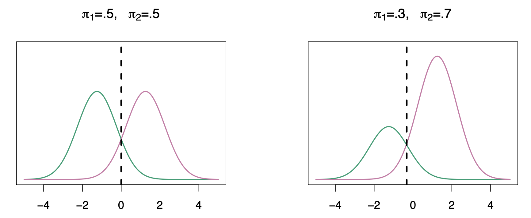
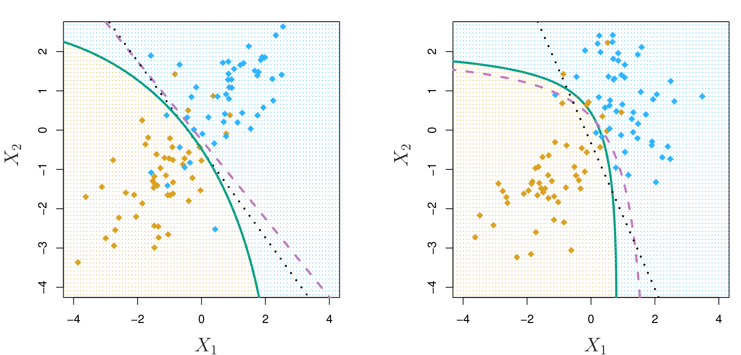
Classify to the Highest Density
![]()
Left-hand plot: single variable X and \(\pi_k f_k(x)\) in the vertical axis for both classes \(k\) equals 1 and \(k\) equals 2. In this case the the pies are the same for both, so anything to the left of zero we classify as as green and anything to the right we classify as as purple.
Right-hand plot: here we have different priors. The probability of \(k = 2\) is 0.7 and and of of \(k= 1\) is 0.3. The decision boundary moved slightly to the left. On the right, we favor the pink class.
Why Discriminant Analysis?
When the classes are well-separated, the parameter estimates for the logistic regression model are surprisingly unstable. Linear discriminant analysis does not suffer from this problem.
If \(n\) is small and the distribution of the predictors \(X\) is approximately normal in each of the classes, the linear discriminant model is again more stable than the logistic regression model.
Linear discriminant analysis is popular when we have more than two response classes, because it also provides low-dimensional views of the data.
Linear Discriminant Analysis when \(p = 1\)
The Gaussian density has the form:
\[
f_k(x) = \frac{1}{\sqrt{2\pi\sigma_k}} e^{-\frac{1}{2} \left( \frac{x - \mu_k}{\sigma_k} \right)^2}
\]
Here \(\mu_k\) is the mean, and \(\sigma_k^2\) the variance (in class \(k\)). We will assume that all the \(\sigma_k = \sigma\) are the same.
Plugging this into Bayes formula, we get a rather complex expression for \(p_k(x) = \Pr(Y = k \mid X = x)\):
\[
p_k(x) = \frac{\pi_k \frac{1}{\sqrt{2\pi\sigma}} e^{-\frac{1}{2} \left( \frac{x - \mu_k}{\sigma} \right)^2}}{\sum_{\ell=1}^K \pi_\ell \frac{1}{\sqrt{2\pi\sigma}} e^{-\frac{1}{2} \left( \frac{x - \mu_\ell}{\sigma} \right)^2}}
\]
Happily, there are simplifications and cancellations.
Discriminant Functions
To classify one observation at the value \(X = x\) into a class, we need to see which of the \(p_k(x)\) is largest. Taking logs, and discarding terms that do not depend on \(k\), we see that this is equivalent to assigning \(x\) to the class with the largest discriminant score:
\[
\delta_k(x) = x \cdot \frac{\mu_k}{\sigma^2} - \frac{\mu_k^2}{2\sigma^2} + \log(\pi_k)
\]
Note that \(\delta_k(x)\) is a linear function of \(x\).
If there are \(K = 2\) classes and \(\pi_1 = \pi_2 = 0.5\), then one can see that the decision boundary is at:
\[
x = \frac{\mu_1 + \mu_2}{2}.
\]
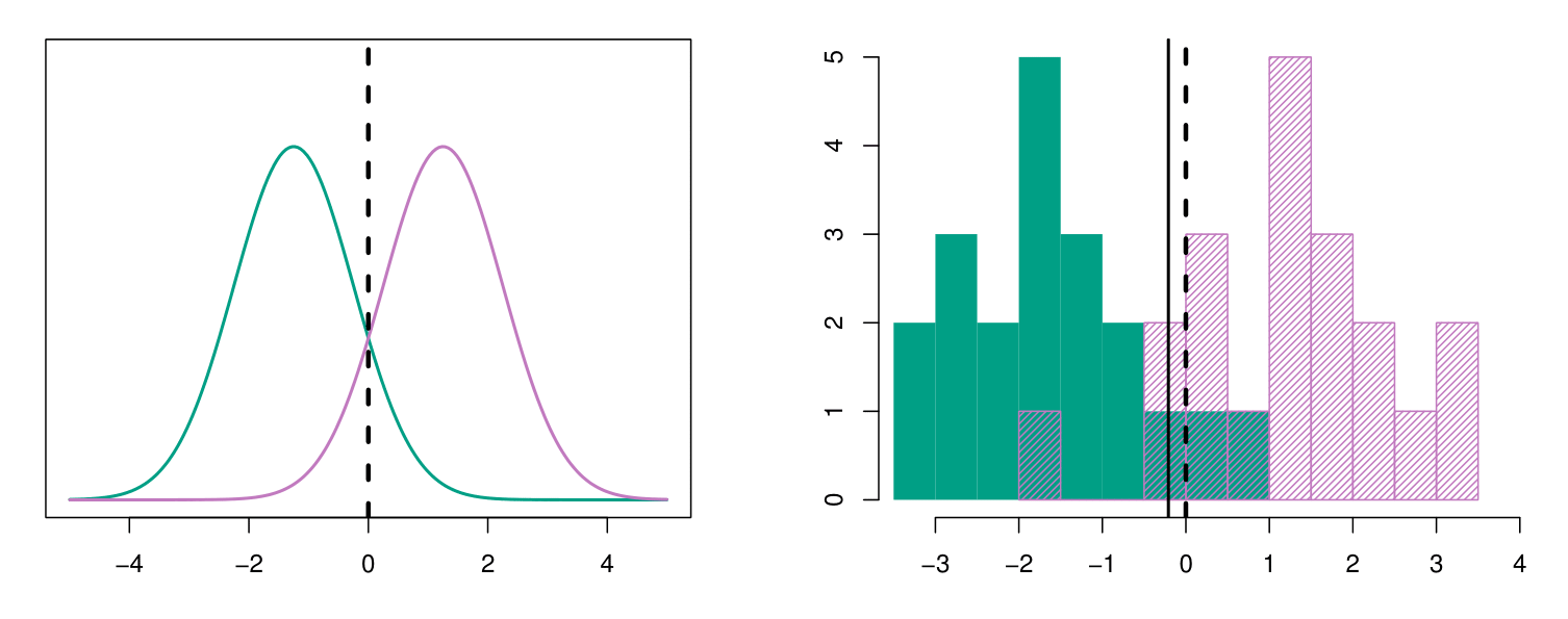
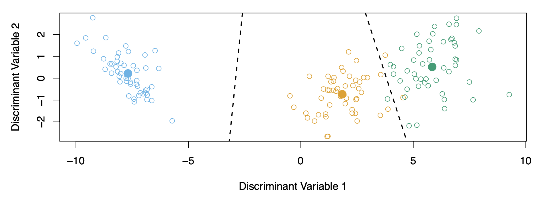
Example: Estimating Parameters for Discriminant Analysis
![]()
Left-Panel: Synthetic population data with \(\mu_1 = -1.5\), \(\mu_2 = 1.5\), \(\pi_1 = \pi_2 = 0.5\), and \(\sigma^2 = 1\).
Typically, we don’t know these parameters; we just have the training data. In that case, we simply estimate the parameters and plug them into the rule.
Right-Panel: histograms of the sample. We see that the estimation provided a decision boundary (black solid line) pretty close to the correct one, the one of the population.
Estimating the Parameters
The prior is the number in each class divided by the total number:
\[
\hat{\pi}_k = \frac{n_k}{n}
\]
The means in each class is the sample mean:
\[
\hat{\mu}_k = \frac{1}{n_k} \sum_{i: y_i = k} x_i
\]
We assume that the variance is the same in each of the classes and so we assume a pooled variance estimate:
\[
\hat{\sigma}^2 = \frac{1}{n - K} \sum_{k=1}^K \sum_{i: y_i = k} (x_i - \hat{\mu}_k)^2
\]
\[
= \sum_{k=1}^K \frac{n_k - 1}{n - K} \cdot \hat{\sigma}_k^2
\]
where \(\hat{\sigma}_k^2 = \frac{1}{n_k - 1} \sum_{i: y_i = k} (x_i - \hat{\mu}_k)^2\) is the usual formula for the estimated variance in the \(k\)-th class.
Naive Bayes
- Assumes features are independent in each class.
- Useful when \(p\) is large, and so multivariate methods like QDA and even LDA break down.
Gaussian Naive Bayes assumes each \(\Sigma_k\) is diagonal:
\[
\begin{aligned}
\delta_k(x) &\propto \log \left[ \pi_k \prod_{j=1}^p f_{kj}(x_j) \right] \\
&= -\frac{1}{2} \sum_{j=1}^p \left[ \frac{(x_j - \mu_{kj})^2}{\sigma_{kj}^2} + \log \sigma_{kj}^2 \right] + \log \pi_k
\end{aligned}
\]
Can be used for mixed feature vectors (qualitative and quantitative). If \(X_j\) is qualitative, replace \(f_{kj}(x_j)\) with the probability mass function (histogram) over discrete categories.
Key Point: Despite strong assumptions, naive Bayes often produces good classification results.
Explanation:
- \(\pi_k\): Prior probability of class \(k\).
- \(f_{kj}(x_j)\): Density function for feature \(j\) in class \(k\).
- \(\mu_{kj}\): Mean of feature \(j\) in class \(k\).
- \(\sigma_{kj}^2\): Variance of feature \(j\) in class \(k\).
Diagonal Covariance Matrix
A diagonal covariance matrix is a special case of the covariance matrix where all off-diagonal elements are zero. This implies that the variables are uncorrelated.
General Form:
For \(p\) variables, a diagonal covariance matrix \(\Sigma\) is represented as:
\[
\Sigma =
\begin{bmatrix}
\sigma_1^2 & 0 & \cdots & 0 \\
0 & \sigma_2^2 & \cdots & 0 \\
\vdots & \vdots & \ddots & \vdots \\
0 & 0 & \cdots & \sigma_p^2
\end{bmatrix}
\]
Properties:
Diagonal Elements (\(\sigma_i^2\)): Represent the variance of each variable \(X_i\).
Off-Diagonal Elements: All equal to zero (\(\text{Cov}(X_i, X_j) = 0\) for \(i \neq j\)), indicating no linear relationship between variables.
A diagonal covariance matrix assumes independence between variables. Each variable varies independently without influencing the others.
Commonly used in simpler models, such as Naive Bayes, where independence is assumed.
Generative Models and Naïve Bayes
Logistic regression models \(\Pr(Y = k | X = x)\) directly, via the logistic function. Similarly, the multinomial logistic regression uses the softmax function. These all model the conditional distribution of \(Y\) given \(X\).
By contrast, generative models start with the conditional distribution of \(X\) given \(Y\), and then use Bayes formula to turn things around:
\[
\Pr(Y = k | X = x) = \frac{\pi_k f_k(x)}{\sum_{l=1}^{K} \pi_l f_l(x)}.
\]
- \(f_k(x)\) is the density of \(X\) given \(Y = k\);
- \(\pi_k = \Pr(Y = k)\) is the marginal probability that \(Y\) is in class \(k\).
Generative Models and Naïve Bayes
- Linear and quadratic discriminant analysis derive from generative models, where \(f_k(x)\) are Gaussian.
- Useful if some classes are well separated. A situation where logistic regression is unstable.
- Naïve Bayes assumes that the densities \(f_k(x)\) in each class factor:
\[
f_k(x) = f_{k1}(x_1) \times f_{k2}(x_2) \times \cdots \times f_{kp}(x_p)
\]
- Equivalently, this assumes that the features are independent within each class.
- Then using Bayes formula:
\[
\Pr(Y = k | X = x) = \frac{\pi_k \times f_{k1}(x_1) \times f_{k2}(x_2) \times \cdots \times f_{kp}(x_p)}{\sum_{l=1}^{K} \pi_l \times f_{l1}(x_1) \times f_{l2}(x_2) \times \cdots \times f_{lp}(x_p)}
\]
Naïve Bayes — Details
Why the independence assumption?
Difficult to specify and model high-dimensional densities.
Much easier to specify one-dimensional densities.
Can handle mixed features:
- If feature \(j\) is quantitative, can model as univariate Gaussian, for example: \(X_j \mid Y = k \sim N(\mu_{jk}, \sigma_{jk}^2).\) We estimate \(\mu_{jk}\) and \(\sigma_{jk}^2\) from the data, and then plug into Gaussian density formula for \(f_{jk}(x_j)\).
- Alternatively, can use a histogram estimate of the density, and directly estimate \(f_{jk}(x_j)\) by the proportion of observations in the bin into which \(x_j\) falls.
- If feature \(j\) is qualitative, can simply model the proportion in each category.
Somewhat unrealistic but extremely useful in many cases.
Despite its simplicity, often shows good classification performance due to reduced variance.
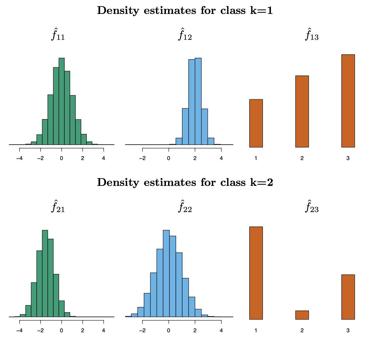
Naïve Bayes — Toy Example
This toy example demonstrates the working of the Naïve Bayes classifier for two classes (\(k = 1\) and \(k = 2\)) and three features (\(X_1, X_2, X_3\)). The goal is to compute the posterior probabilities \(\Pr(Y = 1 \mid X = x^*)\) and \(\Pr(Y = 2 \mid X = x^*)\) for a given observation \(x^* = (0.4, 1.5, 1)\).
The prior probabilities for each class are:
\(\hat{\pi}_1 = \hat{\pi}_2 = 0.5\)
For each feature (\(X_1, X_2, X_3\)), we estimate the class-conditional density functions:
- \(\hat{f}_{11}, \hat{f}_{12}, \hat{f}_{13}\): Densities for \(k = 1\) (class 1).
\(\hat{f}_{11}(0.4) = 0.368 \\\)
\(\hat{f}_{12}(1.5) = 0.484 \\\)
\(\hat{f}_{13}(1) = 0.226 \\\)
- \(\hat{f}_{21}, \hat{f}_{22}, \hat{f}_{23}\): Densities for \(k = 2\) (class 2).
\(\hat{f}_{21}(0.4) = 0.030 \\\)
\(\hat{f}_{22}(1.5) = 0.130 \\\)
\(\hat{f}_{23}(1) = 0.616 \\\)
Naïve Bayes — Toy Example
- Compute Class-Conditional Likelihoods for each class \(k\), the likelihood is computed as the product of the conditional densities for each feature:
\[
\hat{f}_k(x^*) = \prod_{j=1}^3 \hat{f}_{kj}(x_j^*)
\]
\[
\hat{f}_{11}(0.4) = 0.368, \quad \hat{f}_{12}(1.5) = 0.484, \quad \hat{f}_{13}(1) = 0.226
\]
\[
\hat{f}_1(x^*) = 0.368 \times 0.484 \times 0.226 \approx 0.0402
\]
\[
\hat{f}_{21}(0.4) = 0.030, \quad \hat{f}_{22}(1.5) = 0.130, \quad \hat{f}_{23}(1) = 0.616
\]
\[
\hat{f}_2(x^*) = 0.030 \times 0.130 \times 0.616 \approx 0.0024
\]
- Compute Posterior Probabilities using Bayes’ theorem:
\[
\Pr(Y = k \mid X = x^*) = \frac{\hat{\pi}_k \hat{f}_k(x^*)}{\sum_{k=1}^2 \hat{\pi}_k \hat{f}_k(x^*)}
\]
For \(k = 1\): \[
\Pr(Y = 1 \mid X = x^*) = \frac{0.5 \times 0.0402}{(0.5 \times 0.0402) + (0.5 \times 0.0024)} \approx 0.944
\]
For \(k = 2\): \[
\Pr(Y = 2 \mid X = x^*) = \frac{0.5 \times 0.0024}{(0.5 \times 0.0402) + (0.5 \times 0.0024)} \approx 0.056
\]
Key Takeaways:
Naïve Bayes Assumption: The assumption of feature independence simplifies computation by allowing the class-conditional densities to be computed separately for each feature.
Posterior Probabilities: The posterior probability combines the prior (\(\pi_k\)) and the likelihood (\(\hat{f}_k(x^*)\)).
Classification: The observation \(x^*\) is classified as the class with the highest posterior probability (\(Y = 1\)).
Naïve Bayes and GAMs
Naïve Bayes classifier can be understood as a special case of a GAM.
\[
\begin{aligned}
\log \left( \frac{\Pr(Y = k \mid X = x)}{\Pr(Y = K \mid X = x)} \right)
&= \log \left( \frac{\pi_k f_k(x)}{\pi_K f_K(x)} \right) \\
&= \log \left( \frac{\pi_k \prod_{j=1}^p f_{kj}(x_j)}{\pi_K \prod_{j=1}^p f_{Kj}(x_j)} \right) \\
&= \log \left( \frac{\pi_k}{\pi_K} \right) + \sum_{j=1}^p \log \left( \frac{f_{kj}(x_j)}{f_{Kj}(x_j)} \right) \\
&= a_k + \sum_{j=1}^p g_{kj}(x_j),
\end{aligned}
\]
where \(a_k = \log \left( \frac{\pi_k}{\pi_K} \right)\) and \(g_{kj}(x_j) = \log \left( \frac{f_{kj}(x_j)}{f_{Kj}(x_j)} \right)\).
Hence, the Naïve Bayes model is a Generalized Additive Model (GAM):
- The log-odds are expressed as a sum of additive terms.
- \(a_k\): Represents prior influence.
- \(g_{kj}(x_j)\): Represents feature contributions.
Naïve Bayes and GAMs: details
Log-Odds of Posterior Probabilities
The Naïve Bayes classifier starts with the log-odds of the posterior probabilities:
\[
\log \left( \frac{\Pr(Y = k \mid X = x)}{\Pr(Y = K \mid X = x)} \right)
\]
This is the log of the ratio of the probabilities of class \(k\) and a reference class \(K\), given the feature vector \(X = x\).
Naïve Bayes and GAMs: details
Bayes’ Theorem
Using Bayes’ theorem, the posterior probabilities can be expressed as:
\[
\log \left( \frac{\Pr(Y = k \mid X = x)}{\Pr(Y = K \mid X = x)} \right) = \log \left( \frac{\pi_k f_k(x)}{\pi_K f_K(x)} \right)
\]
- \(\pi_k\): Prior probability of class \(k\).
- \(f_k(x)\): Class-conditional density for class \(k\).
Naïve Bayes and GAMs: details
Naïve Bayes Assumption
The Naïve Bayes assumption states that features are conditionally independent given the class:
\[
f_k(x) = \prod_{j=1}^p f_{kj}(x_j)
\]
Substituting this into the equation:
\[
\log \left( \frac{\pi_k f_k(x)}{\pi_K f_K(x)} \right) = \log \left( \frac{\pi_k \prod_{j=1}^p f_{kj}(x_j)}{\pi_K \prod_{j=1}^p f_{Kj}(x_j)} \right)
\]
Naïve Bayes and GAMs: details
Separate the Terms
The terms can now be separated:
\[
\log \left( \frac{\pi_k \prod_{j=1}^p f_{kj}(x_j)}{\pi_K \prod_{j=1}^p f_{Kj}(x_j)} \right)
= \log \left( \frac{\pi_k}{\pi_K} \right) + \sum_{j=1}^p \log \left( \frac{f_{kj}(x_j)}{f_{Kj}(x_j)} \right)
\]
- \(\log \left( \frac{\pi_k}{\pi_K} \right)\): Influence of prior probabilities.
- \(\sum_{j=1}^p \log \left( \frac{f_{kj}(x_j)}{f_{Kj}(x_j)} \right)\): Contribution from each feature.
Naïve Bayes and GAMs: details
Additive Form
Define:
\[
a_k = \log \left( \frac{\pi_k}{\pi_K} \right), \quad g_{kj}(x_j) = \log \left( \frac{f_{kj}(x_j)}{f_{Kj}(x_j)} \right)
\]
The equation becomes:
\[
\log \left( \frac{\Pr(Y = k \mid X = x)}{\Pr(Y = K \mid X = x)} \right) = a_k + \sum_{j=1}^p g_{kj}(x_j)
\]
Generalized Linear Models
Generalized Linear Models
- Linear regression is used for quantitative responses.
- Linear logistic regression is the counterpart for a binary response and models the logit of the probability as a linear model.
- Other response types exist, such as non-negative responses, skewed distributions, and more.
- Generalized linear models provide a unified framework for dealing with many different response types.
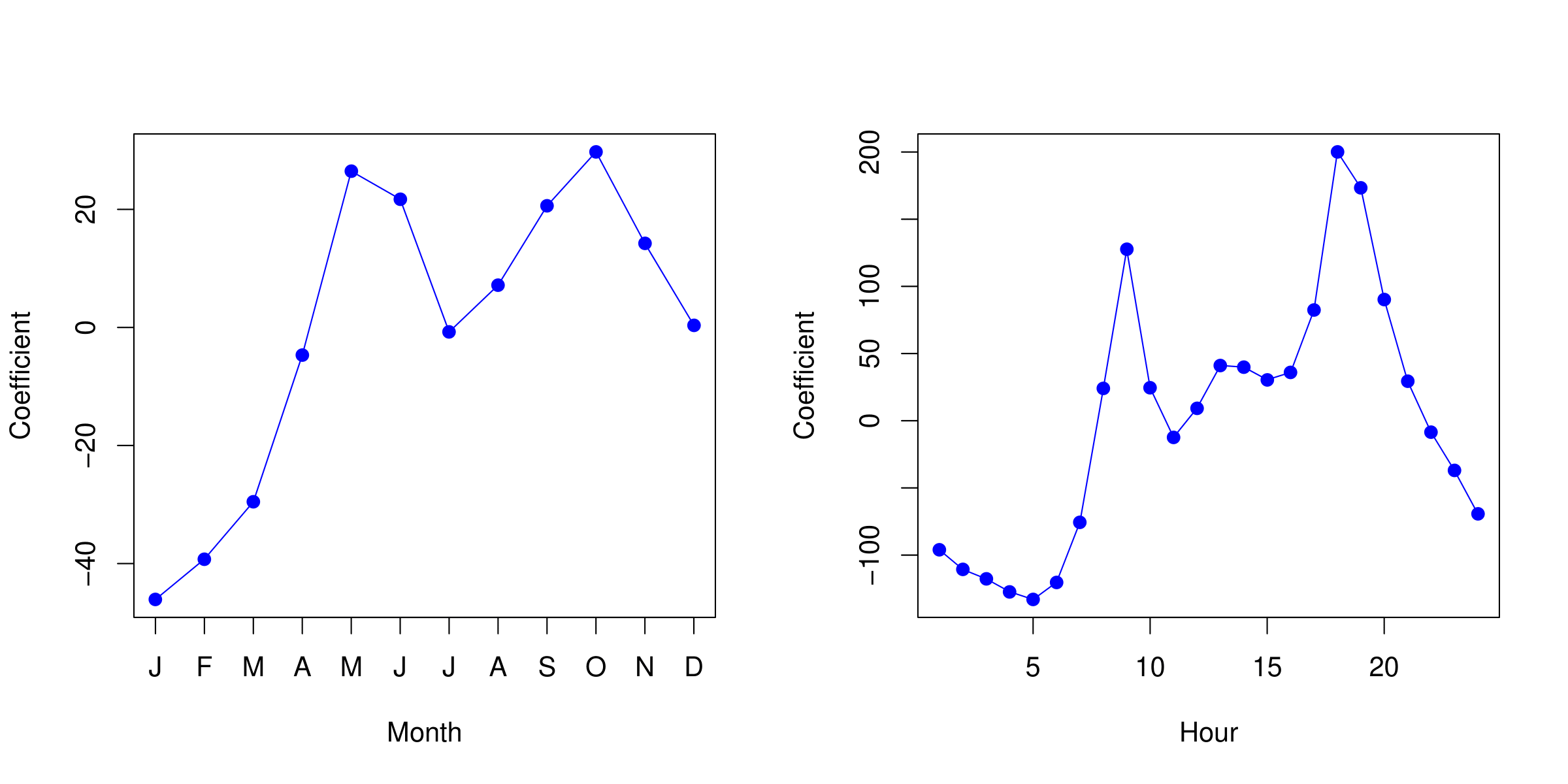
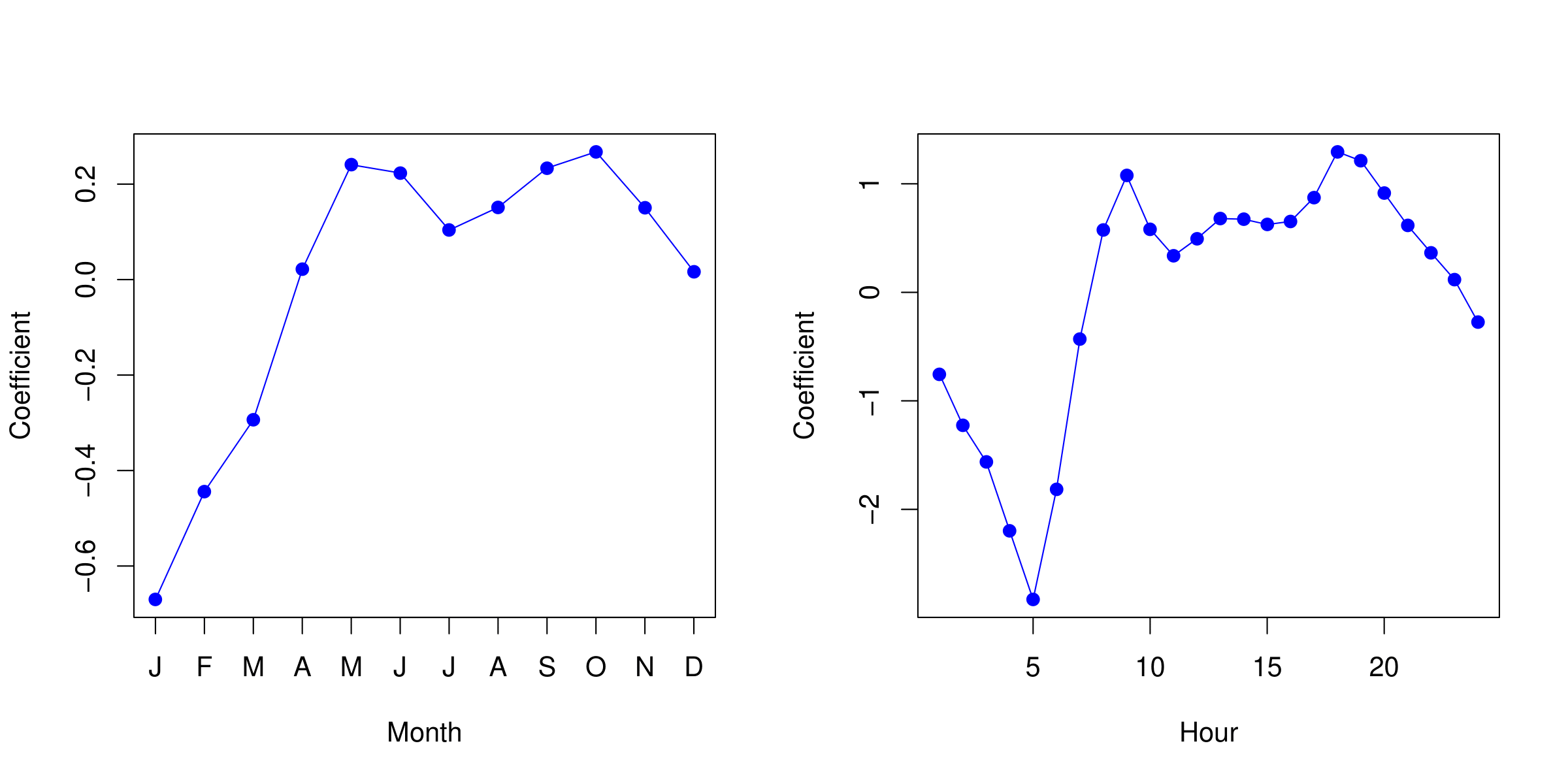
Example: Bikeshare Data
Linear regression with response bikers: number of hourly users in the bikeshare program in Washington, DC.
| Intercept |
73.60 |
5.13 |
14.34 |
0.00 |
| workingday |
1.27 |
1.78 |
0.71 |
0.48 |
| temp |
157.21 |
10.26 |
15.32 |
0.00 |
| weathersit \(cloudy/misty\) |
-12.89 |
1.96 |
-6.56 |
0.00 |
| weathersit \(light rain/snow\) |
-66.49 |
2.97 |
-22.43 |
0.00 |
| weathersit \(heavy rain/snow\) |
-109.75 |
76.67 |
-1.43 |
0.15 |
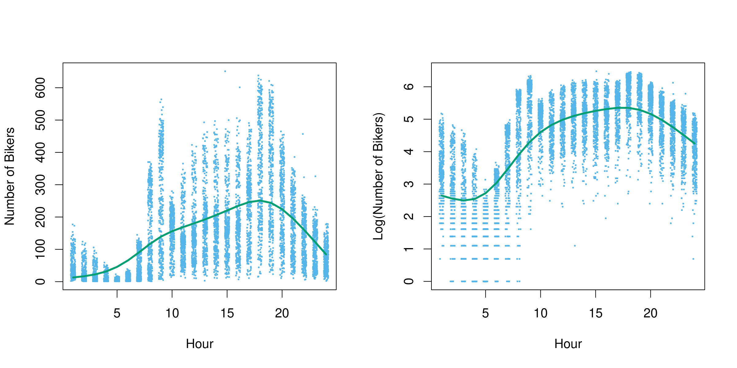
Example: Mean/Variance Relationship
![]()
- Left plot: we see that the variance mostly increases with the mean.
- 10% of a linear model predictions are negative! (not shown here.). However, we know that the response variable,
bikers, is always positive.
- Taking
log(bikers) alleviates this, but is not a good solution. It has its own problems: e.g. predictions are on the wrong scale, and some counts are zero!
Poisson Regression Model
Poisson distribution is useful for modeling counts:
\[
Pr(Y = k) = \frac{e^{-\lambda} \lambda^k}{k!}, \, \text{for } k = 0, 1, 2, \ldots
\]
Mean/variance relationship: \(\lambda = \mathbb{E}(Y) = \text{Var}(Y)\) i.e., there is a mean/variance dependence. When the mean is higher, the variance is higher.
Model with Covariates:
\[
\log(\lambda(X_1, \ldots, X_p)) = \beta_0 + \beta_1 X_1 + \cdots + \beta_p X_p
\]
Or equivalently:
\[
\lambda(X_1, \ldots, X_p) = e^{\beta_0 + \beta_1 X_1 + \cdots + \beta_p X_p}
\]
Automatic positivity: The model ensures that predictions are non-negative by construction.
Example: Poisson Regression on Bikeshare Data
| Intercept |
4.12 |
0.01 |
683.96 |
0.00 |
| workingday |
0.01 |
0.00 |
7.50 |
0.00 |
| temp |
0.79 |
0.01 |
68.43 |
0.00 |
| weathersit \(cloudy/misty\) |
-0.08 |
0.00 |
-34.53 |
0.00 |
| weathersit \(light rain/snow\) |
-0.58 |
0.00 |
-141.91 |
0.00 |
| weathersit \(heavy rain/snow\) |
-0.93 |
0.17 |
-5.55 |
0.00 |
Note: in this case, the variance is somewhat larger than the mean — a situation known as overdispersion. As a result, the p-values may be misleadingly small.
Generalized Linear Models
- We have covered three GLMs: Gaussian, binomial, and Poisson.
- They each have a characteristic link function. This is the transformation of the mean represented by a linear model:
\[
\eta(\mathbb{E}(Y|X_1, X_2, \ldots, X_p)) = \beta_0 + \beta_1 X_1 + \cdots + \beta_p X_p.
\]
The link functions for linear, logistic, and Poisson regression are \(\eta(\mu) = \mu\), \(\eta(\mu) = \log(\mu / (1 - \mu))\), \(\eta(\mu) = \log(\mu)\), respectively.
Each GLM has a characteristic variance function.
The models are fit by maximum likelihood, and model summaries are produced using glm() in R.
Other GLMs include Gamma, Negative-binomial, Inverse Gaussian, and more.