MGMT 17300: Data Mining Lab

Data Wrangling

Professor: Davi Moreira

Overview

Tidy Data
Tidyverse
Data Wrangling

Reshaping Data
Merging Datasets

“Happy families are all alike; every unhappy family is unhappy in its own way.”

— Leo Tolstoy

“Tidy datasets are all alike; every messy dataset is messy in its own way.”

— Hadley Wickham

Tidy Data

Tidy Data vs. Messy Data

In the real world, most data will not be in the format we desire. In this class, we will learn how to process data so that it becomes tidy according to our objectives.

Tidyverse

All the tools we will see are part of the tidyverse, a set of packages for data manipulation.

if(!require(tidyverse)) install.packages("tidyverse")
library(tidyverse)

This set of packages follows principles that are becoming the standard for data analysis in R.

The tidy tools manifesto

Pipe

Pipe

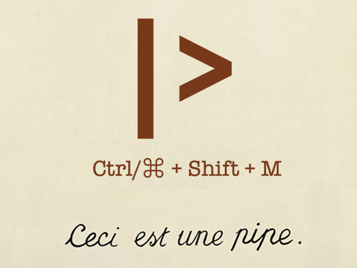
The %>% or |> makes the order of operations clearer, making code easier to read and understand.

# A random vector
x <- c(1:10)

# A simple calculation with complicated code
sum(sqrt(factorial(x)))

# The same calculation with %>% 
x %>% factorial() %>% sqrt() %>% sum()

Data Wrangling

What is Data Wrangling?

Data Wrangling (Data Cleaning / Data Munging):
The process of transforming raw, messy data into a clean and structured format that is ready for analysis.
It often involves:
- Handling missing values
- Correcting inconsistencies
- Reshaping data from wide to long formats (or vice versa)
- Filtering, arranging, and summarizing data

Why is it Important?

Improved Data Quality:
Reliable analyses start with clean, accurate, and consistent data.
Efficiency in Analysis:
Data prepared in a structured and “tidy” format reduces the time spent fixing errors and allows focus on actual insights.
Better Decision Making:
High-quality, well-structured data leads to more meaningful interpretations, stronger conclusions, and actionable insights.

Loading Data

It is advisable to adopt a project-based workflow in your data analysis (Workflow: projects).
Using a consistent project structure optimizes collaboration and sharing of your analysis.
For this lecture, we will use the nycflights13 package, which comes with several related datasets about flights departing from NYC in 2013.

Loading Data

if(!require(nycflights13)) install.packages("nycflights13")
library(nycflights13)

# The main dataset we'll use is flights
flights <- nycflights13::flights

The flights dataset includes information on all US domestic flights departing NYC in 2013. Some key variables include:

year, month, day: date of departure
dep_delay, arr_delay: departure and arrival delays in minutes
carrier: airline carrier
origin and dest: origin and destination airports

Verbs in the Tidyverse

In the tidyverse, we use verbs (functions) that describe step-by-step data manipulation tasks:

filter(): Select rows
arrange(): Sort observations
select() and rename(): Select or rename columns
mutate(): Create new variables
case_when(): Recode variables
summarise() and group_by(): Summarize information
pivot_wider() and pivot_longer(): Reshape data
left_join(): Merge datasets
Combine different steps using the %>% or |>

Selecting Columns with `select()`

The flights dataset has many columns. We can choose only the ones we need:

# Select only a few important columns
flights %>% 
  select(year, month, day, dep_delay, arr_delay)

# Select all columns except a few
flights %>% 
  select(-tailnum, -time_hour)

Selecting Columns with `select()`

# Select columns that start with 'arr'
arr_data <- flights %>% 
  select(starts_with("arr"))

# Rearrange the order of variables
flights_reordered <- flights %>% 
  select(carrier, flight, everything())

Renaming Variables with `rename()`

If we want to rename a variable:

# IMPORTANT: the new name is given first
flights %>% 
  rename(airline = carrier) %>% 
  select(airline, flight, dep_delay)

Creating Variables with `mutate()`

We can create new variables based on existing ones. For example, create a total delay variable:

flights %>% 
  mutate(total_delay = arr_delay + dep_delay) %>% 
  select(year, month, day, carrier, total_delay)

Creating Variables with `transmute()`

transmute() works similarly, but keeps only the newly created variables:

flights %>% 
  transmute(total_delay = arr_delay + dep_delay)

Recoding Variables with `case_when()`

We can recode continuous variables into categories. For example, classify flights as “On Time” if arr_delay <= 0 and “Delayed” otherwise:

flights %>% 
  mutate(status = case_when(
    arr_delay <= 0 ~ "On Time",
    TRUE ~ "Delayed"
  )) %>% 
  select(year, month, day, carrier, arr_delay, status)

Recoding Variables with `case_when()`

We can also have more complex conditions:

flights %>% 
  mutate(delay_category = case_when(
    arr_delay <= 0 ~ "On Time",
    arr_delay <= 30 ~ "Short Delay",
    TRUE ~ "Long Delay"
  )) %>% 
  select(year, month, day, carrier, arr_delay, delay_category)

Selecting Cases with `filter()`

We can select rows based on conditions. For example, flights in January:

flights %>% 
  filter(month == 1)

Or flights in January operated by United Airlines (carrier “UA”):

flights %>% 
  filter(month == 1 & carrier == "UA")

Remembering Logical Operators

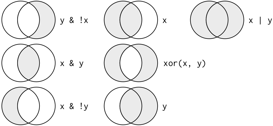
& means AND
| means OR
! means NOT

Selecting Cases with `filter()`

We can store results in a new object using logical operators:

jan_ua_flights <- flights %>% 
  filter(month == 1 & carrier == "UA")

Sorting Observations with `arrange()`

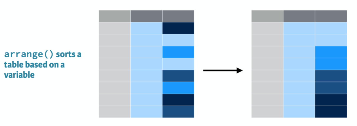
We can sort rows. For example, sort by departure delay ascending:

flights %>% 
  arrange(dep_delay) %>%
  select(carrier, flight, dep_delay)

Sorting Observations with `arrange()`

For descending order:

flights %>% 
  arrange(desc(arr_delay)) %>%
  select(carrier, flight, arr_delay)

Summarizing Information with `summarise()` and `group_by()`

summarise() computes summary statistics. Paired with group_by(), it creates summaries within groups. For example, find the average departure delay by airline carrier:

flights %>% 
  group_by(carrier) %>% 
  summarise(mean_dep_delay = mean(dep_delay, na.rm = TRUE)) %>% 
  drop_na()

Useful functions include mean(), sum(), median(), sd(), n(), and n_distinct().

Other Functions for Grouping

group_by() can be combined with other operations:

flights_group <- flights %>% 
  group_by(month, carrier) %>% 
  summarise(mean_arr_delay = mean(arr_delay, na.rm = TRUE),
            mean_dep_delay = mean(dep_delay, na.rm = TRUE)) %>%
  arrange(mean_arr_delay) %>% 
  ungroup()

flights_group

After grouping and summarizing, always ungroup() to return to the normal structure.

Reshaping Data

Reshaping Data with `pivot_wider()` and `pivot_longer()`

Let’s create a summary and then reshape it. For example, find the average arrival delay by carrier and month, then pivot to a wide format.

Our data is currently in long format.

`pivot_wider()`: from long to wide

# Create a summary of mean arrival delay by carrier and month
delay_summary <- flights %>%
  group_by(carrier, month) %>%
  summarise(mean_arr_delay = mean(arr_delay, na.rm = TRUE)) %>%
  ungroup()

# Pivot wider: carriers in rows, months in columns
delay_wide <- delay_summary %>% 
  pivot_wider(names_from = month, values_from = mean_arr_delay)

delay_wide

`pivot_longer()`: from wide to long

If we want to go back to the long format:

delay_long <- delay_wide %>% 
  pivot_longer(cols = -carrier, names_to = "month", values_to = "mean_arr_delay")

delay_long

Merging Datasets

“There are two certainties in life: death and bad merges”

Merging Datasets

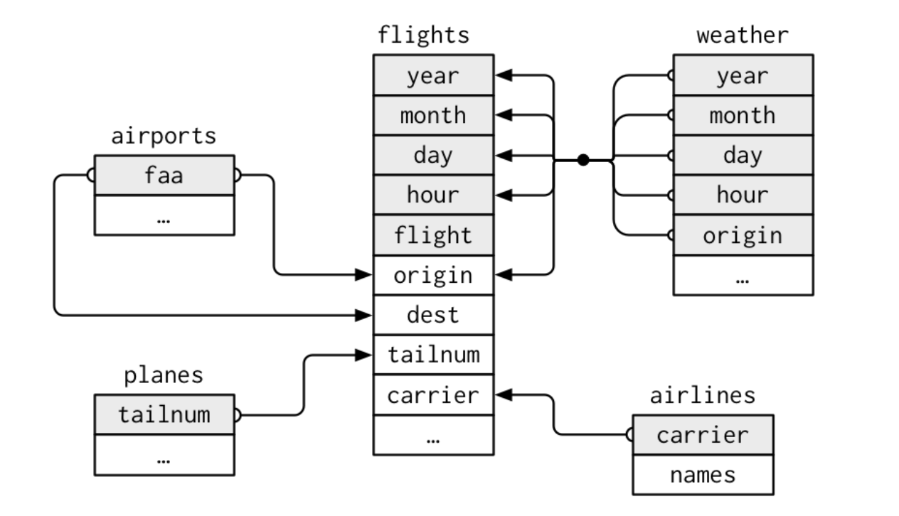
The flights dataset can be connected to others:

flights connects to planes by: tailnum.
flights connects to airlines by: carrier.
flights connects to airports by: origin and dest.
flights connects to weather by: origin, year, month, day, hour.

Commands for Joining

Commands for Joining `full_join()`

Commands for Joining `inner_join()`

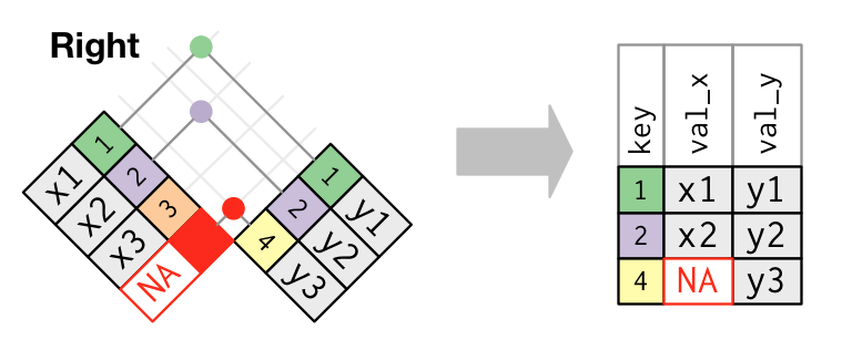
Commands for Joining `right_join()`

Commands for Joining `left_join()`

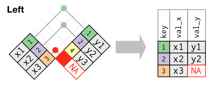
Merging Datasets: Example

For instance, to attach airline names to flights:

flights_with_names <- flights %>% 
  left_join(airlines, by = "carrier")

head(flights_with_names)

Additional Material

Some interesting resources:

Summary

Using the %>% or |> to streamline code
Selecting and renaming columns
Filtering and sorting rows
Creating and recoding variables
Summarizing groups of observations
Reshaping data from long to wide and back
Joining multiple datasets for richer analysis

MGMT 17300: Data Mining Lab

Overview

Tidy Data

Tidy Data vs. Messy Data

Tidyverse

Tidyverse

Pipe

Pipe

Data Wrangling

What is Data Wrangling?

Why is it Important?

Loading Data

Loading Data

Verbs in the Tidyverse

Selecting Columns with select()

Selecting Columns with select()

Renaming Variables with rename()

Creating Variables with mutate()

Creating Variables with mutate()

Creating Variables with transmute()

Recoding Variables with case_when()

Recoding Variables with case_when()

Selecting Cases with filter()

Selecting Cases with filter()

Remembering Logical Operators

Selecting Cases with filter()

Sorting Observations with arrange()

Sorting Observations with arrange()

Sorting Observations with arrange()

Summarizing Information with summarise() and group_by()

Other Functions for Grouping

Reshaping Data

Reshaping Data with pivot_wider() and pivot_longer()

pivot_wider(): from long to wide

pivot_longer(): from wide to long

Merging Datasets

Merging Datasets

Commands for Joining

Commands for Joining full_join()

Commands for Joining inner_join()

Commands for Joining right_join()

Commands for Joining left_join()

Merging Datasets: Example

Additional Material

Summary

Summary

Thank you!

Selecting Columns with `select()`

Selecting Columns with `select()`

Renaming Variables with `rename()`

Creating Variables with `mutate()`

Creating Variables with `mutate()`

Creating Variables with `transmute()`

Recoding Variables with `case_when()`

Recoding Variables with `case_when()`

Selecting Cases with `filter()`

Selecting Cases with `filter()`

Selecting Cases with `filter()`

Sorting Observations with `arrange()`

Sorting Observations with `arrange()`

Sorting Observations with `arrange()`

Summarizing Information with `summarise()` and `group_by()`

Reshaping Data with `pivot_wider()` and `pivot_longer()`

`pivot_wider()`: from long to wide

`pivot_longer()`: from wide to long

Commands for Joining `full_join()`

Commands for Joining `inner_join()`

Commands for Joining `right_join()`

Commands for Joining `left_join()`