MGMT 47400: Predictive Analytics

Linear Regression

Professor: Davi Moreira

Overview

• Recap

• Linear Regression

• Simple Linear Regression

• Multiple Linear Regression

• Considerations in the Regression Model

  • Qualitative Predictors

• Extensions of the Linear Model

  • Interactions
  • Hierarchy

• Non-linear effects of predictors

This lecture content is inspired by and replicates the material from An Introduction to Statistical Learning.

Recap

What is Statistical Learning?

A framework to learn the relationship between predictors \(X\) and an outcome \(Y\) for prediction and inference, using parametric (e.g., linear/logistic regression) and non-parametric methods (e.g., trees, kNN).

What is the difference between supervised and unsupervised learning?

Supervised: learn \(f: X \to Y\) from labeled data to predict/explain \(Y\).
Unsupervised: find structure in \(X\) without labels (e.g., clustering, dimensionality reduction).

What is the curse of dimensionality?

With many features/predictors, data become sparse; distances degrade, required sample size grows rapidly, and generalization deteriorates, especially for local/partitioning methods.

What is the difference between overfitting and underfitting?

Overfitting: too flexible; captures noise (high variance); low training error, poor test error.
Underfitting: too simple; misses signal (high bias); high error on both train and test.

Why assess accuracy on test data rather than training data?

Training accuracy is optimistically biased (evaluated on seen data). Test accuracy estimates out-of-sample performance and reveals overfitting.

Participation

• In pairs, ask AI:

  • In the context of Statistical Learning, what is the fundamental difference between a regression problem and a classification problem in supervised learning, based on the nature of the outcome variable?

• Present the response you got to your right/left classmate. Do your understanding converge?

• Submit your participation response.

Linear Regression

Linear Regression

• Linear regression is a simple approach to supervised learning. It assumes that the dependence of \(Y\) on \(X_1, X_2, \ldots, X_p\) is linear.

• True regression functions are never linear!

• Although it may seem overly simplistic, linear regression is extremely useful both conceptually and practically.

Linear Regression for the Advertising Data

Consider the advertising data shown:

Suppose that, in our job as business analysts, we are asked to suggest, based on this data, a marketing plan for next year that will result in high product sales. What information would be useful in order to provide such a recommendation?

The Marketing Plan: Guiding Questions

1. Is there a relationship between advertising budget and sales?
   Our first goal is to determine whether the data provide evidence of an association between advertising expenditure and sales. If the evidence is weak, one might argue that no money should be spent on advertising.

2. How strong is the relationship between advertising budget and sales?
   Assuming a relationship exists, how strong is it? Does knowledge of the advertising budget provide a lot of information about product sales?

3. Which media are associated with sales?
   Are all three media—TV, radio, and newspaper—associated with sales, or just one or two? We must separate the individual contribution of each medium to sales when money is spent on all three.

4. How large is the association between each medium and sales?
   For every dollar spent on a particular medium, by what amount will sales increase? How accurately can we predict this amount?

5. How accurately can we predict future sales?
   For any given level of television, radio, or newspaper advertising, what is our prediction for sales, and what is the accuracy of this prediction?

6. Is the relationship linear?
   If the relationship between advertising expenditure and sales is approximately linear, then linear regression is appropriate. If not, we may need to transform the predictor(s) or the response so that linear regression can be used.

7. Is there synergy among the advertising media?
   Perhaps spending $50,000 on television advertising and $50,000 on radio advertising is associated with higher sales than allocating $100,000 to either television or radio individually. In marketing, this is known as a synergy effect; in statistics, it is called an interaction effect.

Simple Linear Regression

Simple Linear Regression using a single predictor \(X\)

• We assume a model:

\[ Y = \beta_0 + \beta_1X + \epsilon, \]

where \(\beta_0\) and \(\beta_1\) are two unknown constants that represent the intercept and slope, also known as coefficients or parameters, and \(\epsilon\) is the error term.

• Given some estimates \(\hat{\beta}_0\) and \(\hat{\beta}_1\) for the model coefficients, we predict future sales using:

\[ \hat{y} = \hat{\beta}_0 + \hat{\beta}_1x, \]

where \(\hat{y}\) indicates a prediction of \(Y\) on the basis of \(X = x\). The hat symbol denotes an estimated value.

Estimation of the parameters by least squares

• Let \(\hat{y}_i = \hat{\beta}_0 + \hat{\beta}_1 x_i\) be the prediction for \(Y\) based on the \(i\)th value of \(X\). Then \(e_i = y_i - \hat{y}_i\) represents the \(i\)th residual.

• We define the residual sum of squares (RSS) as:

\[ RSS = e_1^2 + e_2^2 + \cdots + e_n^2, \]

or equivalently as:

\[ RSS = (y_1 - \hat{\beta}_0 - \hat{\beta}_1 x_1)^2 + (y_2 - \hat{\beta}_0 - \hat{\beta}_1 x_2)^2 + \cdots + (y_n - \hat{\beta}_0 - \hat{\beta}_1 x_n)^2. \]

• The least squares approach selects the estimators \(\hat{\beta}_0\) and \(\hat{\beta}_1\) to minimize the RSS. The minimizing values can be shown to be:

\[ \hat{\beta}_1 = \frac{\sum_{i=1}^n (x_i - \bar{x})(y_i - \bar{y})}{\sum_{i=1}^n (x_i - \bar{x})^2}, \quad \hat{\beta}_0 = \bar{y} - \hat{\beta}_1 \bar{x}, \]

where \(\bar{y} \equiv \frac{1}{n} \sum_{i=1}^n y_i\) and \(\bar{x} \equiv \frac{1}{n} \sum_{i=1}^n x_i\) are the sample means.

Example: Advertising Data

The least squares fit for the regression of sales onto TV is shown. In this case a linear fit captures the essence of the relationship, although it is somewhat deficient in the left of the plot

Assessing the Accuracy of the Coefficient Estimates

• The standard error of an estimator reflects how it varies under repeated sampling:

\[ SE(\hat{\beta}_1)^2 = \frac{\sigma^2}{\sum_{i=1}^n (x_i - \bar{x})^2}, \quad SE(\hat{\beta}_0)^2 = \sigma^2 \left[ \frac{1}{n} + \frac{\bar{x}^2}{\sum_{i=1}^n (x_i - \bar{x})^2} \right]. \]

where \(\sigma^2 = Var(\epsilon)\)

• These standard errors can be used to compute confidence intervals. A 95% confidence interval is defined as a range of values such that with 95% probability, the range will contain the true unknown value of the parameter. It has the form:

\[ \hat{\beta}_1 \pm 2 \cdot SE(\hat{\beta}_1). \]

• There is approximately a 95% chance that the interval:

\[ \left[ \hat{\beta}_1 - 2 \cdot SE(\hat{\beta}_1), \hat{\beta}_1 + 2 \cdot SE(\hat{\beta}_1) \right] \]

will contain the true value of \(\beta_1\) (under a scenario where we obtained repeated samples like the present sample).

• For the advertising data, the 95% confidence interval for \(\beta_1\) is:

\[ [0.042, 0.053]. \]

Hypothesis Testing

• Standard errors can be used to perform hypothesis tests on coefficients. The most common hypothesis test involves testing the null hypothesis:

\[ H_0: \text{There is no relationship between } X \text{ and } Y \] versus the alternative hypothesis:

\[ H_A: \text{There is some relationship between } X \text{ and } Y. \]

• Mathematically, this corresponds to testing:

\[ H_0: \beta_1 = 0 \] versus:

\[ H_A: \beta_1 \neq 0, \]

since if \(\beta_1 = 0\), then the model reduces to \(Y = \beta_0 + \epsilon\), and \(X\) is not associated with \(Y\).

Hypothesis Testing

• To test the null hypothesis (\(H_0\)), compute a \(t\)-statistic as follows:

\[ t = \frac{\hat{\beta}_1 - 0}{SE(\hat{\beta}_1)}. \]

• The \(t\)-statistic follows a \(t\)-distribution with \(n - 2\) degrees of freedom under the null hypothesis (\(\beta_1 = 0\)).

• Using statistical software, we can compute the \(p\)-value to determine the likelihood of observing a \(t\)-statistic as extreme as the one calculated.

Results for the Advertising Data

Variable	Coefficient	Std. Error	t-statistic	p-value
Intercept	7.0325	0.4578	15.36	< 0.0001
TV	0.0475	0.0027	17.67	< 0.0001

Assessing the Overall Accuracy of the Model

• Residual Standard Error (RSE):

\[ RSE = \sqrt{\frac{1}{n-2} RSS} = \sqrt{\frac{1}{n-2} \sum_{i=1}^n (y_i - \hat{y}_i)^2} \] where the Residual Sum of Square (RSS) is \(\sum_{i=1}^n (y_i - \hat{y})^2\).

• \(R^2\), the fraction of variance explained:

\[ R^2 = \frac{TSS - RSS}{TSS} = 1 - \frac{RSS}{TSS}, \quad TSS = \sum_{i=1}^n (y_i - \bar{y})^2 \] where TSS is the Total Sums of Squares.

• It can be shown that in this Simple Linear Regression setting that \(R^2 = r^2\), where \(r\) is the correlation between X and Y:

\[ r = \frac{\sum_{i=1}^n (x_i - \bar{x})(y_i - \bar{y})}{\sqrt{\sum_{i=1}^n (x_i - \bar{x})^2 \sum_{i=1}^n (y_i - \bar{y})^2}} \]

Advertising Data Results

Key metrics for model accuracy:

Quantity	Value
Residual Standard Error	3.26
R²	0.612
F-statistic	312.1

Multiple Linear Regression

Multiple Linear Regression

• Here our model is

\[ Y = \beta_0 + \beta_1 X_1 + \beta_2 X_2 + \cdots + \beta_p X_p + \epsilon, \]

• We interpret \(\beta_j\) as the average effect on \(Y\) of a one-unit increase in \(X_j\), holding all other predictors fixed.

• In the advertising example, the model becomes

\[ \text{sales} = \beta_0 + \beta_1 \times \text{TV} + \beta_2 \times \text{radio} + \beta_3 \times \text{newspaper} + \epsilon. \]

Interpreting Regression Coefficients

• The ideal scenario is when the predictors are uncorrelated — a balanced design:
  • Each coefficient can be estimated and tested separately.
  • Interpretations such as “a unit change in \(X_j\) is associated with a \(\beta_j\) change in \(Y\), while all the other variables stay fixed” are possible.
• Correlations amongst predictors cause problems:
  • The variance of all coefficients tends to increase, sometimes dramatically.
  • Interpretations become hazardous — when \(X_j\) changes, everything else changes.
• Claims of causality should be avoided for observational data.

Estimation and Prediction for Multiple Regression

• Given estimates \(\hat{\beta}_0, \hat{\beta}_1, \ldots, \hat{\beta}_p\), we can make predictions using the formula:

\[ \hat{y} = \hat{\beta}_0 + \hat{\beta}_1x_1 + \hat{\beta}_2x_2 + \cdots + \hat{\beta}_px_p. \]

• We estimate \(\beta_0, \beta_1, \ldots, \beta_p\) as the values that minimize the sum of squared residuals:

\[ \text{RSS} = \sum_{i=1}^n \left( y_i - \hat{y}_i \right)^2 = \sum_{i=1}^n \left( y_i - \hat{\beta}_0 - \hat{\beta}_1x_{i1} - \hat{\beta}_2x_{i2} - \cdots - \hat{\beta}_px_{ip} \right)^2. \]

• This is done using standard statistical software. The values \(\hat{\beta}_0, \hat{\beta}_1, \ldots, \hat{\beta}_p\) that minimize RSS are the multiple least squares regression coefficient estimates.

Results for Advertising Data

Regression Coefficients

Predictor	Coefficient	Std. Error	t-statistic	p-value
Intercept	2.939	0.3119	9.42	< 0.0001
TV	0.046	0.0014	32.81	< 0.0001
radio	0.189	0.0086	21.89	< 0.0001
newspaper	-0.001	0.0059	-0.18	0.8599

Correlations

Predictor	TV	radio	newspaper	sales
TV	1.0000	0.0548	0.0567	0.7822
radio		1.0000	0.3541	0.5762
newspaper			1.0000	0.2283
sales				1.0000

Some Important Questions

1. Is at least one of the predictors \(X_1, X_2, \dots, X_p\) useful in predicting the response?

2. Do all the predictors help to explain \(Y\), or is only a subset of the predictors useful?

3. How well does the model fit the data?

4. Given a set of predictor values, what response value should we predict, and how accurate is our prediction?

Is at Least One Predictor Useful?

For the first question, we can use the F-statistic:

\[ F = \frac{(TSS - RSS) / p}{RSS / (n - p - 1)} \sim F_{p, n-p-1} \]

Quantity	Value
Residual Standard Error	1.69
\(R^2\)	0.897
F-statistic	570

The F-statistic is huge and it’s p-value is less than \(.0001\). This says that there’s a strong association of the predictors on the outcome variable.

Deciding on the Important Variables

Deciding on the Important Variables

• The most direct approach is called all subsets or best subsets regression:

  • Compute the least squares fit for all possible subsets.

  • Choose between them based on some criterion that balances training error with model size.

• However, we often can’t examine all possible models since there are (\(2^p\)) of them.

  • For example, when (p = 40), there are over a billion models!

• Instead, we need an automated approach that searches through a subset of them.

Forward Selection

• Begin with the null model — a model that contains an intercept but no predictors.

• Fit \(p\) Simple Linear Regressions and add to the null model the variable that results in the lowest RSS.

• Add to that model the variable that results in the lowest RSS amongst all two-variable models.

• Continue until some stopping rule is satisfied:

  • For example, when all remaining variables have a p-value above some threshold.

Backward Selection

• Start with all variables in the model.

• Remove the variable with the largest p-value — that is, the variable that is the least statistically significant.

• The new (\(p - 1\))-variable model is fit, and the variable with the largest p-value is removed.

• Continue until a stopping rule is reached:

  • For instance, we may stop when all remaining variables have a significant p-value defined by some significance threshold.

Model Selection

• We will discuss other criterias for choosing an “optimal” member in the path of models produced by forward or backward stepwise selection, including:

  • Mallow’s \(C_p\)

  • Akaike information criterion (AIC)

  • Bayesian information criterion (BIC)

  • Adjusted \(R^2\)

  • Cross-validation (CV)

Other Considerations in the Regression Model

Qualitative Predictors

• Some predictors are qualitative, taking discrete values.

• Categorical predictors can be represented using factor variables.

• Qualitative variables: Student (Student Status), Status (Marital Status), Own (Owns a House).

Credit Card Data

Credit Card Data

Suppose we investigate differences in credit card balance between those who own a house and those who do not, ignoring the other variables. We create a new variable:

\[ x_i = \begin{cases} 1 & \text{if } i\text{th person owns a house} \\ 0 & \text{if } i\text{th person does not own a house} \end{cases} \]

Resulting model:

\[ y_i = \beta_0 + \beta_1 x_i + \epsilon_i = \begin{cases} \beta_0 + \beta_1 + \epsilon_i & \text{if } i\text{th person owns a house} \\ \beta_0 + \epsilon_i & \text{if } i\text{th person does not own a house.} \end{cases} \]

Credit Card Data

Results for the model:

Predictor	Coefficient	Std. Error	t-statistic	p-value
Intercept	509.80	33.13	15.389	< 0.0001
Own [Yes]	19.73	46.05	0.429	0.6690

We see the coefficient is 19.73, but it’s not significant. The p value is 0.66 which is not significant (> 0.05). So, owing a house don’t generally means a higher credit card balance than not owing one.

Qualitative Predictors with More Than Two Levels

With more than two levels, we create additional dummy variables.

For example, for the `region`` variable, we create two dummy variables:

\[ x_{i1} = \begin{cases} 1 & \text{if i-th person is from the South} \\ 0 & \text{if i-th person is not from the South} \end{cases} \]

\[ x_{i2} = \begin{cases} 1 & \text{if i-th person is from the West} \\ 0 & \text{if i-th person is not from the West} \end{cases} \]

Qualitative Predictors

Both variables can be used in the regression equation to obtain the model:

\[ y_i = \beta_0 + \beta_1 x_{i1} + \beta_2 x_{i2} + \epsilon_i = \begin{cases} \beta_0 + \beta_1 + \epsilon_i & \text{if i-th person is from the South} \\ \beta_0 + \beta_2 + \epsilon_i & \text{if i-th person is from the West}\\ \beta_0 + \epsilon_i & \text{if i-th person is from the East (baseline)} \end{cases} \]

Note: There will always be one fewer dummy variable than the number of levels. The level with no dummy variable — East in this example — is known as the baseline.

Results for Ethnicity

Term	Coefficient	Std. Error	t-statistic	p-value
Intercept	531.00	46.32	11.464	< 0.0001
ethnicity \(South\)	-18.69	65.02	-0.287	0.7740
ethnicity \(West\)	-12.50	56.68	-0.221	0.8260

The coefficient -18.69 compares South to East and that’s not significant. Likewise, the West to East is also not significant.

Note: the choice of the baseline does not affect the fit of the model. The residual sum of sum of squares will be the same no matter which category we chose as the baseline. At its turn, the p-values will potentially change as we change the baseline category.

Extensions of the Linear Model

Interactions

In our previous analysis of the Advertising data, we assumed that the effect on sales of increasing one advertising medium is independent of the amount spent on the other media.

For example, the linear model

\[ \widehat{\text{sales}} = \beta_0 + \beta_1 \times \text{TV} + \beta_2 \times \text{radio} + \beta_3 \times \text{newspaper} \]

states that the average effect on sales of a one-unit increase in TV is always \(\beta_1\), regardless of the amount spent on radio.

Interactions

• But suppose that spending money on radio advertising actually increases the effectiveness of TV advertising, so that the slope term for TV should increase as radio increases.

• In this situation, given a fixed budget of $100,000, spending half on radio and half on TV may increase sales more than allocating the entire amount to either TV or radio.

• In marketing, this is known as a synergy effect, and in statistics, it is referred to as an interaction effect.

Interaction in Advertising Data

• When levels of TV or radio are low, true sales are lower than predicted.

• Splitting advertising between TV and radio underestimates sales.

Modeling Interactions

Model takes the form:

\[ \text{sales} = \beta_0 + \beta_1 \times \text{TV} + \beta_2 \times \text{radio} + \beta_3 \times (\text{radio} \times \text{TV}) + \epsilon \]

Term	Coefficient	Std. Error	t-statistic	p-value
Intercept	6.7502	0.248	27.23	< 0.0001
TV	0.0191	0.002	12.70	< 0.0001
radio	0.0289	0.009	3.24	0.0014
TV × radio	0.0011	0.000	20.73	< 0.0001

Interpretation

• The results in this table suggest that interactions are important.The p-value for the interaction term TV \(\times\) radio is extremely low, indicating that there is strong evidence for ( H_A : \(\beta_3 \neq 0\)).

• The ( \(R^2\) ) for the interaction model is 96.8%, compared to only 89.7% for the model that predicts sales using TV and radio without an interaction term.

• This means that (\(\frac{96.8 - 89.7}{100 - 89.7}\)) = 69% of the variability in sales that remains after fitting the additive model has been explained by the interaction term.

• The coefficient estimates in the table suggest that an increase in TV advertising of $1,000 is associated with increased sales of (\(\hat{\beta}_1 + \hat{\beta}_3 \times \text{radio}\)) \(\times 1000 = 19 + 1.1 \times \text{radio} \text{ units}.\)

• An increase in radio advertising of $1,000 will be associated with an increase in sales of (\(\hat{\beta}_2 + \hat{\beta}_3 \times \text{TV}\)) \(\times 1000 = 29 + 1.1 \times \text{TV} \text{ units}.\)

Hierarchy

• Sometimes it is the case that an interaction term has a very small p-value, but the associated main effects (in this case, TV and radio) do not.

• The hierarchy principle:

  • If we include an interaction in a model, we should also include the main effects, even if the p-values associated with their coefficients are not significant.

• The rationale for this principle is that interactions are hard to interpret in a model without main effects.

• Specifically, the interaction terms also contain main effects, if the model has no main effect terms.

Interactions Between Qualitative and Quantitative Variables

Consider the Credit data set, and suppose that we wish to predict balance using income (quantitative) and student (qualitative).

Without an interaction term, the model takes the form:

\[ \text{balance}_i \approx \beta_0 + \beta_1 \times \text{income}_i + \begin{cases} \beta_2 & \text{if } i^\text{th} \text{ person is a student} \\ 0 & \text{if } i^\text{th} \text{ person is not a student} \end{cases} \]

\[ = \beta_1 \times \text{income}_i + \begin{cases} \beta_0 + \beta_2 & \text{if } i^\text{th} \text{ person is a student} \\ \beta_0 & \text{if } i^\text{th} \text{ person is not a student} \end{cases} \]

With Interactions, It Takes the Form

\[ \text{balance}_i \approx \beta_0 + \beta_1 \times \text{income}_i + \begin{cases} \beta_2 + \beta_3 \times \text{income}_i & \text{if student} \\ 0 & \text{if not student} \end{cases} \]

\[ = \begin{cases} (\beta_0 + \beta_2) + (\beta_1 + \beta_3) \times \text{income}_i & \text{if student} \\ \beta_0 + \beta_1 \times \text{income}_i & \text{if not student} \end{cases} \]

Visualizing Interactions

• Left: no interaction between income and student.
• Right: with an interaction term between income and student.

Non-linear effects of predictors

Non-linear effects of predictors

Polynomial regression on Auto data

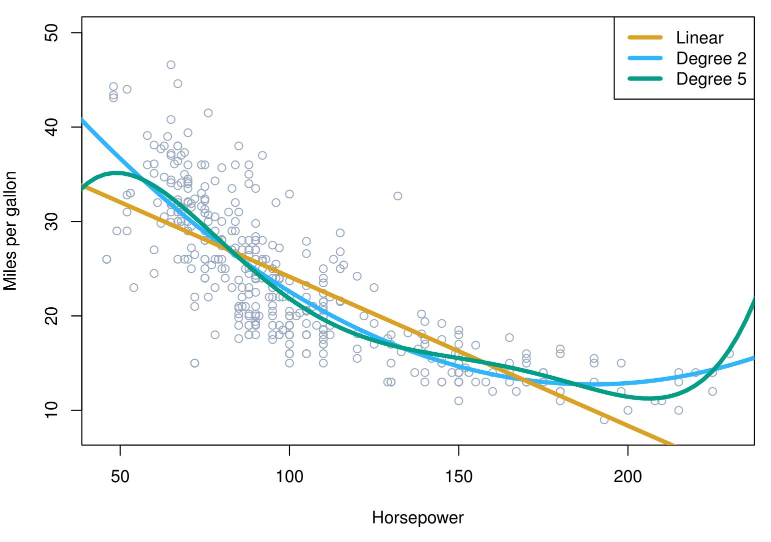
Non-linear regression results

The figure suggests that the following model

\[ mpg = \beta_0 + \beta_1 \times horsepower + \beta_2 \times horsepower^2 + \epsilon \]

may provide a better fit.

	Coefficient	Std. Error	t-statistic	p-value
Intercept	56.9001	1.8004	31.6	< 0.0001
horsepower	-0.4662	0.0311	-15.0	< 0.0001
\(\text{horsepower}^2\)	0.0012	0.0001	10.1	< 0.0001

What we did not cover

• Outliers
• Non-constant variance of error terms
• High leverage points
• Collinearity

Generalizations of the Linear Model

• In much of the rest of the course we discuss methods that expand the scope of linear models and how they are fit:

  • Classification problems: logistic regression, support vector machines.

  • Non-linearity: kernel smoothing, splines, generalized additive models; nearest neighbor methods.

  • Interactions: Tree-based methods, bagging, random forests, boosting (these also capture non-linearities).

  • Regularized fitting: Ridge regression and lasso.

The Marketing Plan: Answers

The Marketing Plan: Answers

1.Is there a relationship between sales and advertising budget?

Fit a multiple regression of sales on TV, radio, and newspaper, and test

\[ H_0:\ \beta_{\text{TV}}=\beta_{\text{radio}}=\beta_{\text{newspaper}}=0. \]

Using the \(F\)-statistic, the very small \(p\)-value indicates clear evidence of a relationship between advertising and sales.

2. How strong is the relationship?

Two accuracy measures:

• RSE: estimates the standard deviation of the response from the population regression line. For Advertising, RSE \(\approx\) 3.26. In other words, actual sales in each market deviate from the true regression line by approximately 3,260 units, on average. In the data set, the mean value of sales over all markets is approximately 14,000 units, and so the percentage error is 3,260/14,000 = 23 %.

• \(R^2\) (variance explained): records the percentage of variability in the response that is explained by the predictors. Predictors explain ~90% of the variance in sales.

3. Which media are associated with sales?

Check \(p\)-values for each predictor’s \(t\)-statistic. The \(p\)-values for TV and radio are low, but newspaper is not, suggesting only TV and radio are related to sales.

4. How large is the association between each medium and sales?

We used SEs to build 95% CIs for coefficients related to TV, Radio, Newspaper.

TV and radio intervals are narrow and far from 0, which means a strong evidence of association. Newspaper CI includes 0, not significant given TV and radio.

5. How accurately can we predict future sales?

Accuracy depends on whether predicting an individual response, \(Y=f(X)+\epsilon\), or the average response, \(f(X)\).

• Individual \(\rightarrow\) prediction interval

• Average \(\rightarrow\) confidence interval

Prediction intervals are always wider because they include irreducible error uncertainty from \(\epsilon\).

The Marketing Plan: Answers

6. Is the relationship linear?

Residual plots help diagnose nonlinearity; linear relationships yield residuals with no pattern. Transformations can accommodate nonlinearity within linear regression.

7. Is there synergy among the advertising media?

Standard linear regression assumes additivity. This is interpretable but may be unrealistic. An interaction term allows non-additive relationships; a small \(p\)-value on the interaction indicates synergy. For Advertising, adding an interaction increases \(R^2\) substantially — from ~90% to almost 97%.

Summary

Summary

• Linear Regression:

  • A foundational supervised learning method.
  • Assumes a linear relationship between predictors (\(X\)) and the response (\(Y\)).
  • Useful for both prediction and understanding relationships.

• Simple vs. Multiple Regression:

  • Simple regression: one predictor.
  • Multiple regression: multiple predictors.

• Key Metrics:

  • Residual Standard Error (RSE), \(R^2\), and F-statistic.
  • Confidence intervals and hypothesis testing for coefficients.

• Qualitative Predictors:

  • Use dummy variables for categorical predictors.
  • Interpret results based on chosen baselines.

• Interactions:

  • Models with interaction terms (e.g., \(X_1 \times X_2\)) capture synergistic effects.

• Non-linear Effects:

  • Polynomial regression accounts for curvature in data.

• Challenges:

  • Multicollinearity, outliers, high leverage points.
  • Overfitting vs. underfitting: balance flexibility and interpretability.

Thank you!