MGMT 17300: Data Mining Lab

Evaluating Predictive Model Performance

Professor: Davi Moreira

August 01, 2024

Overview

• Lesson Exercise Review

• Lesson Question!

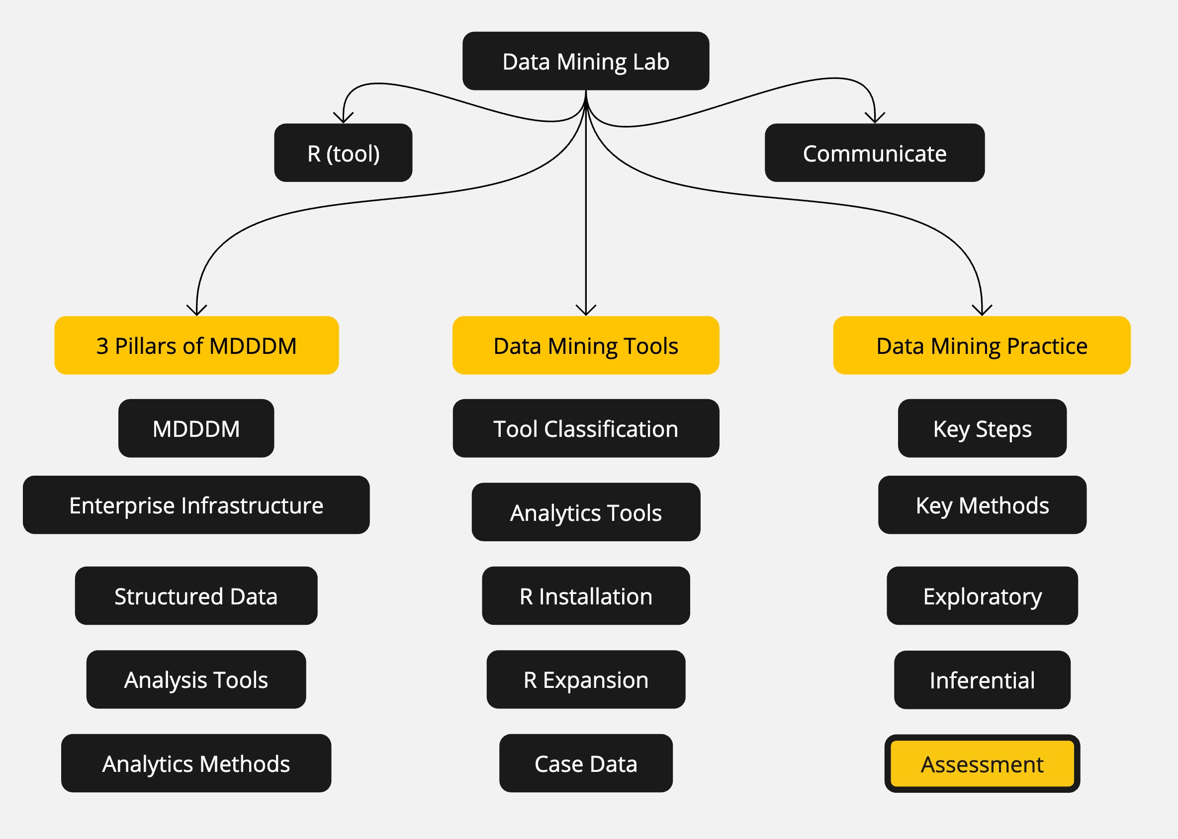
• Course Learning Milestones

• The 8 Key Steps of a Data Mining Project

• Multiple Regression Model
• Model Interpretation
• Making predictions
• Evaluating Predictive Model Performance

Lesson Exercises Review

Lesson Question!

Course Learning Milestones

Course Learning Milestones

The 8 Key Steps of a Data Mining Project

The 8 Key Steps of a Data Mining Project

Goal Setting

1. Define the project’s goal
   

Data Understanding

2. Acquire analysis tools
   
3. Prepare data
   
4. Data summarization
   
5. Data visualization
   

Insights

6. Data mining modeling
   
7. Model validation
   
8. Interpretation and implementation

Making predictions with a predictive model

Best Subset Selection

Method: Use the regsubsets() function from the leaps package to evaluate all possible combinations of predictors and identify the best model. This method guarantees that the best subset of predictors is selected according to a chosen criterion (e.g., adjusted \(R^2\), AIC, BIC).

Selection: This method ensures an exhaustive search of all possible combinations, providing the best model for each subset size.

library(leaps)

# Fit the best subset model
best_model <- regsubsets(mpg ~ ., data = mtcars, nbest = 1)

# Extract the summary of the model
best_model_summary <- summary(best_model)

# Extract metrics
bic_values <- best_model_summary$bic

# Find the best model indices based on each criterion
best_bic_index <- which.min(bic_values)

# Display the best models based on the chosen criteria

cat("\nBest model based on BIC includes:\n")
print(coef(best_model, best_bic_index))

Result: The regsubsets() function outputs the best subset of predictors for each model size, allowing you to compare and choose the optimal model based on adjusted \(R^2\), BIC, or other criteria.

In our case now, we are concerned with the optimal model for prediction, so we are using BIC as our criteria.

Cross-Validation

Method: Use k-fold cross-validation to assess the predictive performance of the model. This method helps evaluate how the model generalizes to unseen data.

Selection: Choose the model with better cross-validation metrics (e.g., lower mean squared error).

library(caret)

# Define the cross-validation method
trainControl <- trainControl(method = "cv", number = 10)

# Train the model based on adjusted R-squared criteria
original_model <- train(mpg ~ hp, data = mtcars, method = "lm", trControl = trainControl)
# print(original_model)

# Train the model based on BIC criteria
model_bic <- train(mpg ~ wt + qsec + am, data = mtcars, method = "lm", trControl = trainControl)
# print(model_bic)

# Compare RMSE, R-squared, and MAE (Mean Absolute Error) for both models
#cat("\nComparison of Prediction Performance:\n")
performance_comparison <- rbind(
  "original_model" = original_model$results[, c("RMSE", "Rsquared", "MAE")],
  "Model_bic" = model_bic$results[, c("RMSE", "Rsquared", "MAE")]
)
print(performance_comparison)

Cross-Validation: output

• RMSE (Root Mean Squared Error):
  • Represents the standard deviation of prediction errors.
  • Lower values indicate better performance (predictions are closer to actual values).
• R-squared:
  • Indicates how well the independent variables explain the variability of the dependent variable.
  • Higher values (closer to 1) suggest better explanatory power.
• MAE (Mean Absolute Error):
  • Measures the average magnitude of errors in predictions.
  • Lower values indicate more accurate predictions.

Cross-Validation: Conclusion

original_model:

• Better at explaining variability (higher R-squared).

• Slightly higher prediction error (RMSE and MAE).

model_bic:

• More accurate predictions (lower RMSE and MAE).

• Explains less variability (lower R-squared).

Recommendation

• Choose original_model: If the goal is to maximize explanation of variability in mpg.

• Choose Model_bic: If the goal is to minimize prediction error for better accuracy.

Final Choice: Depends if the analysis objective prioritize explanatory power or prediction accuracy.

Making predictions with a predictive model

Now that we have our prediction model, let’s see an example on how can we use it for prediction.

To predict mpg with our model we need to have data regarding our independent variables. To do so, let’s split our original dataset:

library(caret)

set.seed(123)  # for reproducibility
splitIndex <- createDataPartition(mtcars$mpg, p = 0.8, list = FALSE)
training_data <- mtcars[splitIndex, ]
testing_data <- mtcars[-splitIndex, ]

Making predictions with a predictive model

We run the model with our training_data and predict the mpg values using our testing_data.

# models
model_bic <- lm(mpg ~ wt + qsec + am, data = training_data)
original_model <- lm(mpg ~ hp, data = training_data)

# predictions
predictions_bic <- predict(model_bic, newdata = testing_data)
predictions_original <- predict(original_model, newdata = testing_data)

Evaluating Predictive Model Performance

By combining our predicted results into our original dataset, we can check in which extent we were able to predict the actual mpg values:

# Combine actual and predicted values into a long format
library(tidyr)

# Combine data into one long-format object
plot_data <- data.frame(
  actual = testing_data$mpg,
  predicted_bic = predictions_bic,
  predicted_original = predictions_original
) %>%
  pivot_longer(
    cols = starts_with("predicted"),
    names_to = "model",
    values_to = "predicted"
  )

plot_data

Evaluating Predictive Model Performance

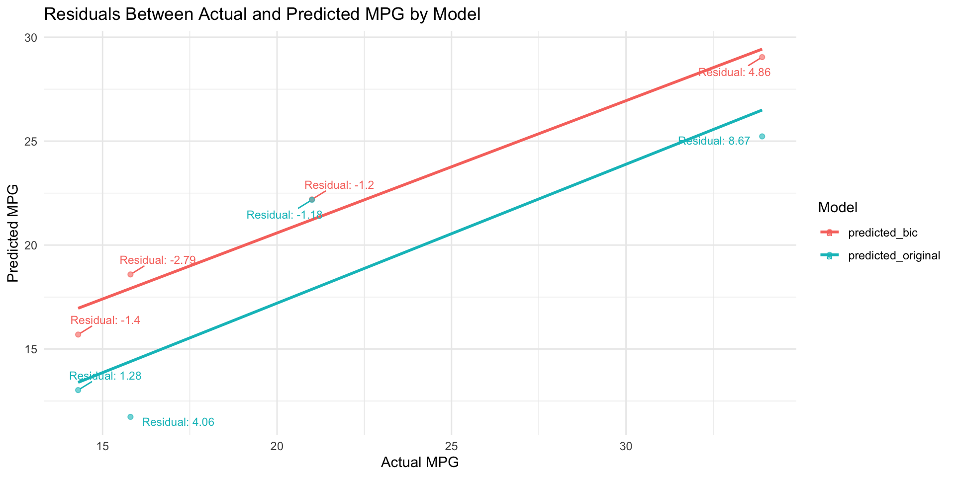
We can plot a scatter plot with the actual mpg values on the x-axis and predicted mpg values on the y-axis.

# Load ggrepel for better label placement
library(ggrepel)

# Create a scatter plot with residuals labeled and prediction lines
ggplot(plot_data, aes(x = actual, y = predicted, color = model)) +
  geom_point(alpha = 0.6) +  # Scatter plot of actual vs predicted
  geom_smooth(method = "lm", formula = y ~ x, se = FALSE) +  # Linear trend lines
  geom_text_repel(
    aes(label = paste0("Residual: ", round(actual - predicted, 2))),  # Residual as label
    size = 3, 
    max.overlaps = 10,  # Controls the maximum number of overlapping labels
    box.padding = 0.5,  # Padding around the text box
    point.padding = 0.2  # Padding around the point
  ) + 
  labs(
    x = "Actual MPG", 
    y = "Predicted MPG", 
    color = "Model", 
    title = "Residuals Between Actual and Predicted MPG by Model"
  ) +
  theme_minimal()

Summary

Summary

Main Takeaways from this lecture:

• Choose the model with higher adjusted R-squared for explanatory power.

• Opt for lower RMSE and MAE if prediction accuracy is the main objective.

Thank you!