MGMT 17300: Data Mining Lab
Predictive Model Interpretations and Predictions
August 01, 2024
Overview
Lesson Exercise Review
Lesson Question!
Course Learning Milestones
The 8 Key Steps of a Data Mining Project
- Multiple Regression Model
- Model Interpretation
- Making predictions
Lesson Exercises Review
Lesson Question!
Course Learning Milestones
Course Learning Milestones

The 8 Key Steps of a Data Mining Project
The 8 Key Steps of a Data Mining Project
Goal Setting
- Define the project’s goal
Data Understanding
- Acquire analysis tools
- Prepare data
- Data summarization
- Data visualization
Insights
- Data mining modeling
- Model validation
- Interpretation and implementation
Multiple Regression Model
Precision and Accuracy
Precision: Refers to the consistency or reliability of the model’s predictions.
Accuracy: Refers to how close the model’s predictions are to the true values.
In the context of regression:
- High Precision, Low Accuracy: Predictions are consistent but biased.
- High Precision, High Accuracy: Predictions are both consistent and valid.
- Low Precision, Low Accuracy: Predictions are neither consistent nor valid.
- Low Precision, High Accuracy: Predictions are valid on average but have high variability.
To achieve high precision and high accuracy, we need to meet the model assumptions.
Motivation: Controlling for a Variable
- Puzzle: What is the effect of education on income?
- Y: Income
- X: Education
- Objective: X \(\rightarrow\) Y
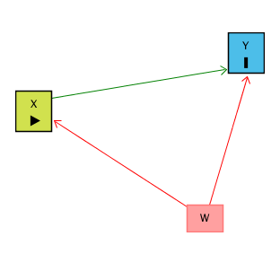
- Challenge: X \(\leftarrow\) W \(\rightarrow\) Y
- W: IQ (Intelligence)
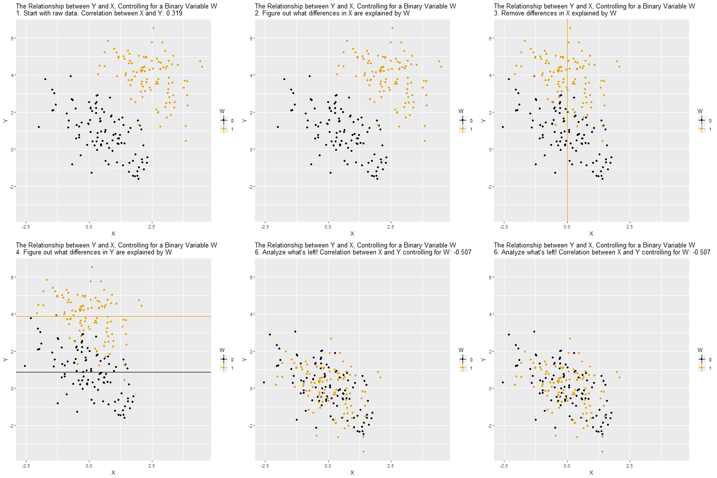
- Solution: Control for W
Motivation: Controlling for a Variable

Source: Causal Inference Animated Plots
Motivation: Controlling for a Variable

Source: Causal Inference Animated Plots
Omitted Variables (Confounders)
One of the most common errors in observational studies (besides selection bias and information bias — classification or measurement error);
It occurs when we suggest that the explanation for something is “confounded” with the effect of another variable;
For example, “the sun rose because the rooster crowed,” and not because of Earth’s rotation.
How to Address Omitted Variable Bias?
Be well-versed in the literature;
Select good control variables for your model;
That is, perform a multiple regression model.
Multiple Regression
Regression analysis involving two or more independent variables (x’s).
This subject area, called multiple regression analysis, enables us to consider more independent variables (factors) and thus obtain better estimates of the relationship than are possible with simple linear regression.
Multiple Regression Model
The equation that describes how the dependent variable \(y\) is related to the independent variables \(x_1, x_2, \ldots x_p\) and an error term \(\epsilon\) is:
\[ y = \beta_0 + \beta_1 x_1 + \beta_2 x_2 + \dots + \beta_p x_p + \epsilon \]
Where:
\(\beta_0, \beta_1, \beta_2, \dots, \beta_p\) are the unknown parameters.
\(\epsilon\) is a random variable called the error term with the same assumptions as in simple regression (Normality, zero mean, constant variance, independence).
\(p\) is the number of independent variables (dimension or complexity of the model).
Multiple Regression Equation
The equation that describes how the mean value of \(y\) is related to \(x_1, x_2, \ldots x_p\) is:
\[ E(y) = \beta_0 + \beta_1 x_1 + \beta_2 x_2 + \dots + \beta_p x_p \]
\(\beta_1, \ldots, \beta_p\) measure the marginal effects of the respective independent variables.
For example, \(\beta_1\) is the change in \(E(y)\) corresponding to a 1-unit increase in \(x_1\), when all other independent variables are held constant or when we control for all other independent variables.
Estimated Multiple Regression Equation
\[ \hat{y} = b_0 + b_1 x_1 + b_2 x_2 + \dots + b_p x_p \]
A simple random sample is used to compute sample slopes \(b_0, b_1, b_2, \dots, b_p\) that are used as the point estimators of the population slopes \(\beta_0, \beta_1, \beta_2, \dots, \beta_p\).
Hence, \(\hat{y}\) estimates \(E(Y)\).
Multiple Regression Model Example
Objective
- Analyze the relationship between multiple predictors and miles per gallon (
mpg). - Build a multiple linear regression model to predict
mpgbased on:- Horsepower (
hp) - Weight (
wt) - Transmission Type (
am) - Engine Type (
vs) - Number of Cylinders (
cyl)
- Horsepower (
Variables Used
- mpg: Miles per gallon (Dependent Variable).
- hp: Gross horsepower.
- wt: Weight (1000 lbs).
- am: Transmission (0 = automatic, 1 = manual).
- vs: Engine type (0 = V-shaped, 1 = straight).
- cyl: Number of cylinders.
Data Structure
'data.frame':   32 obs. of  6 variables:
 $ mpg: num  21 21 22.8 21.4 18.7 18.1 14.3 24.4 22.8 19.2 ...
 $ hp : num  110 110 93 110 175 105 245 62 95 123 ...
 $ wt : num  2.62 2.88 2.32 3.21 3.44 ...
 $ am : num  1 1 1 0 0 0 0 0 0 0 ...
 $ vs : num  0 0 1 1 0 1 0 1 1 1 ...
 $ cyl: num  6 6 4 6 8 6 8 4 4 6 ...
Summary Statistics
Converting Categorical Variables
Checking for Missing Values
- Observation: No missing values in the selected variables.
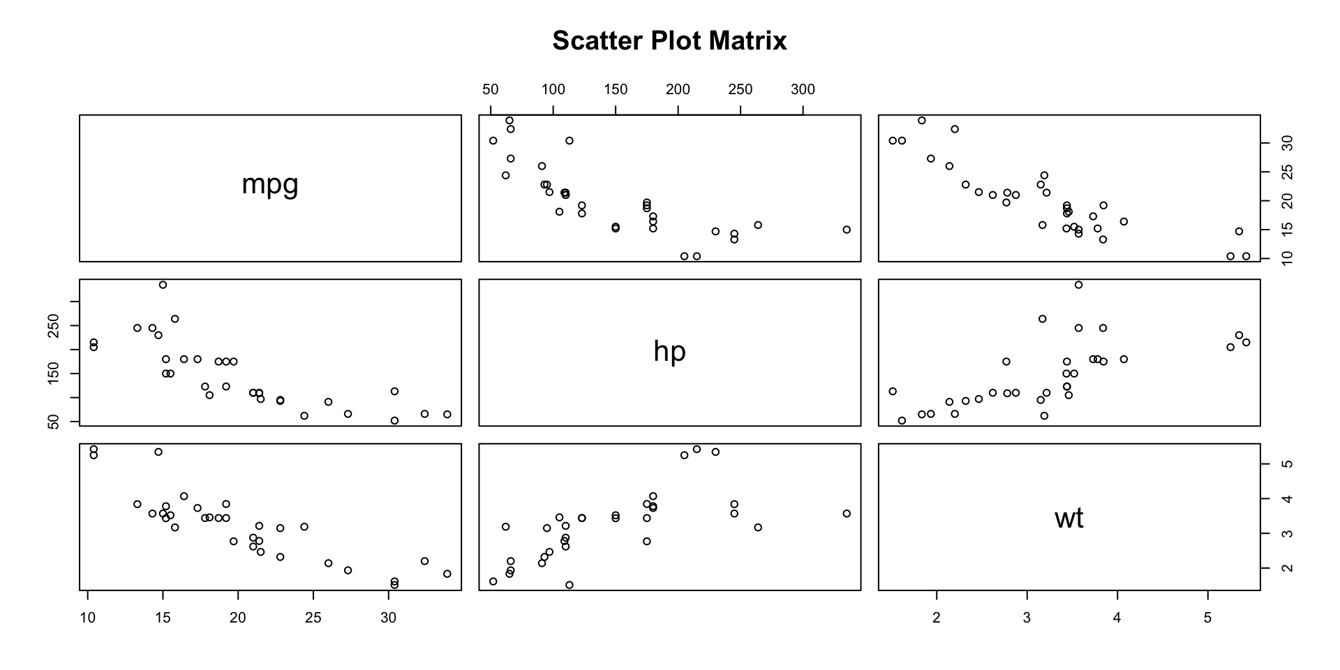
Visualizing Relationships: Pairwise Scatter Plots
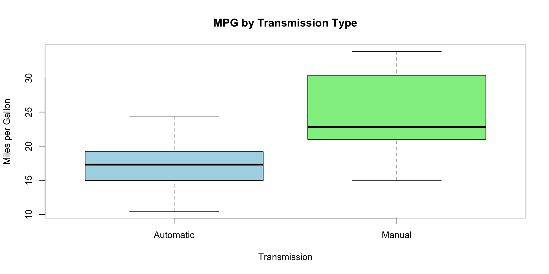
Boxplots for Categorical Variables
Fitting the Multiple Regression Model
Call:
lm(formula = mpg ~ hp + wt + am + vs + cyl, data = mtcars)

Residuals:
    Min      1Q  Median      3Q     Max
-4.3405 -1.2158  0.0046  0.9389  4.6354

Coefficients:
            Estimate Std. Error t value Pr(>|t|)
(Intercept) 31.18461    3.42002   9.118    2e-09 ***
hp          -0.03475    0.01382  -2.515   0.0187 *
wt          -2.37337    0.88763  -2.674   0.0130 *
amManual     2.70384    1.59850   1.691   0.1032
vsStraight   1.99000    1.76018   1.131   0.2690
cyl6        -2.09011    1.62868  -1.283   0.2112
cyl8         0.29098    3.14270   0.093   0.9270
---
Signif. codes:  0 '***' 0.001 '**' 0.01 '*' 0.05 '.' 0.1 ' ' 1

Residual standard error: 2.397 on 25 degrees of freedom
Multiple R-squared:  0.8724,    Adjusted R-squared:  0.8418
F-statistic: 28.49 on 6 and 25 DF,  p-value: 5.064e-10
Interpreting the Coefficients
- Intercept (\(\beta_0\)): Expected
mpgwhen all predictors are at reference levels or zero. - hp: Change in
mpgper unit increase in horsepower, holding other variables constant. - wt: Change in
mpgper 1000 lbs increase in weight, holding other variables constant. - am: Difference in
mpgbetween manual and automatic transmission. - vs: Difference in
mpgbetween straight and V-shaped engines. - cyl: Effect of the number of cylinders on
mpg.
Interpreting the Results
Significant Predictors
- hp and wt: Generally significant predictors of
mpg. - am: Transmission type may have a significant effect.
- vs and cyl: Assess their p-values to determine significance.
- hp and wt: Generally significant predictors of
Evaluating the Model
Adjusted R-squared: Measures the proportion of variance in
mpgexplained by the model, adjusted for the number of predictors.F-statistic: Tests the overall significance of the model.
p-values: Assess the significance of individual predictors.
Making predictions with a predictive model
Best Subset Selection
Method: Use the regsubsets() function from the leaps package to evaluate all possible combinations of predictors and identify the best model. This method guarantees that the best subset of predictors is selected according to a chosen criterion (e.g., adjusted \(R^2\), AIC, BIC).
Selection: This method ensures an exhaustive search of all possible combinations, providing the best model for each subset size.
library(leaps)

# Fit the best subset model
best_model <- regsubsets(mpg ~ ., data = mtcars, nbest = 1)

# Extract the summary of the model
best_model_summary <- summary(best_model)

# Extract metrics
bic_values <- best_model_summary$bic

# Find the best model indices based on each criterion
best_bic_index <- which.min(bic_values)

# Display the best models based on the chosen criteria

cat("\nBest model based on BIC includes:\n")
print(coef(best_model, best_bic_index))
Result: The regsubsets() function outputs the best subset of predictors for each model size, allowing you to compare and choose the optimal model based on adjusted \(R^2\), BIC, or other criteria.
In our case now, we are concerned with the optimal model for prediction, so we are using BIC as our criteria.
Cross-Validation
Method: Use k-fold cross-validation to assess the predictive performance of the model. This method helps evaluate how the model generalizes to unseen data.
Selection: Choose the model with better cross-validation metrics (e.g., lower mean squared error).
library(caret)

# Define the cross-validation method
trainControl <- trainControl(method = "cv", number = 10)

# Train the model based on adjusted R-squared criteria
original_model <- train(mpg ~ hp + wt + am + vs + cyl, data = mtcars, method = "lm", trControl = trainControl)
# print(original_model)

# Train the model based on BIC criteria
model_bic <- train(mpg ~ wt + qsec + am, data = mtcars, method = "lm", trControl = trainControl)
# print(model_bic)

# Compare RMSE, R-squared, and MAE (Mean Absolute Error) for both models
#cat("\nComparison of Prediction Performance:\n")
performance_comparison <- rbind(
  "original_model" = original_model$results[, c("RMSE", "Rsquared", "MAE")],
  "Model_bic" = model_bic$results[, c("RMSE", "Rsquared", "MAE")]
)
print(performance_comparison)
Cross-Validation: output
- RMSE (Root Mean Squared Error):
- Represents the standard deviation of prediction errors.
- Lower values indicate better performance (predictions are closer to actual values).
- R-squared:
- Indicates how well the independent variables explain the variability of the dependent variable.
- Higher values (closer to 1) suggest better explanatory power.
- MAE (Mean Absolute Error):
- Measures the average magnitude of errors in predictions.
- Lower values indicate more accurate predictions.
Cross-Validation: Conclusion
original_model:
Better at explaining variability (higher R-squared).
Slightly higher prediction error (RMSE and MAE).
model_bic:
More accurate predictions (lower RMSE and MAE).
Explains less variability (lower R-squared).
Recommendation
Choose original_model: If the goal is to maximize explanation of variability in
mpg.Choose Model_bic: If the goal is to minimize prediction error for better accuracy.
Final Choice: Depends if the analysis objective prioritize explanatory power or prediction accuracy.
Making predictions with a predictive model
Now that we have our prediction model, let’s see an example on how can we use it for prediction.
To predict mpg with our model we need to have data regarding our independent variables. To do so, let’s split our original dataset:
Making predictions with a predictive model
We run the model with our training_data and predict the mpg values usin our testing_data.
Making predictions with a predictive model
By combining our predicted results into our original dataset, we can check in which extent we were able to predict the actual mpg values:
Making predictions with a predictive model
We can plot a scatter plot with the actual mpg values on the x-axis and predicted mpg values on the y-axis.
The red line represents a linear regression line that helps us see how well our predictions align with the actual data.
Summary
Summary
Main Takeaways from this lecture:
- Model Evaluation and Precision:
- Precision: Consistency of model predictions.
- Accuracy: Closeness of predictions to true values.
- Aim for high precision and high accuracy by meeting model assumptions.
- Controlling for Variables:
- Importance of controlling for confounders.
- Use multiple regression to control for potential confounding variables.
- Strategies for Model Selection:
- Identify predictors with low p-values (< 0.05) to determine their significance.
- Use Adjusted R-Squared, AIC/BIC, and F-Tests for model comparison.
- Multicollinearity: Check with VIF and address high VIF (> 10).
- Best Subset Selection: Use
regsubsets()to find the best combination of predictors. - Cross-Validation: Evaluate models using RMSE, R-squared, and MAE.
- Key Recommendations:
- Choose the model with higher adjusted R-squared for explanatory power.
- Opt for lower RMSE and MAE if prediction accuracy is the main objective.
- Balance between complexity and performance using AIC/BIC and other metrics.
Thank you!
Data Mining Lab

